How to use PowerPivot in Excel: The Ultimate Guide

Power Pivot is an add-in first introduced in Excel 2010 and now a staple part of the modern Excel. It has changed the way that we can work with and manipulate large volumes of data in Excel.

In this article, we will not only answer the question of what is Power Pivot? But also why and how to use PowerPivot with real business use cases.

What is Power Pivot & why is it useful?

Although an Excel worksheet can handle 1,048,576 rows of data. In reality, it can struggle as you get to 100,000 or even before that depending on what you have in your workbook.

Power Pivot enables us to work with big data beyond the 1,048,576 limitation and still produce smaller, leaner and faster workbooks than a standard PivotTable.

It does this by loading the data into the internal data model of Excel and not onto a worksheet. Relationships can then be created between the different tables of data. No more VLOOKUPs to pull data together into one big list.

We can then create PivotTables based on this model to analyze multiple tables of data.

You can also use a powerful formula language in Power Pivot called DAX. This stands for Data Analysis Expressions.

The DAX language is vast and enables us to perform more complex calculations than we can do with a standard PivotTable.

So what is Power Pivot? It is really a combination of using PivotTables and DAX calculations with the internal data model of Excel for analysis of big data.

Check out this short video that explains why we need Power Pivot:

In this guide, we'll cover:

• How to get and install the Power Pivot add-in
• How to import CVS files into the Data Model
• Viewing the Data Model in Power Pivot
• Creating relationships between the tables
• Creating a Pivot Table from the Data Model
• Using DAX to create Measure
• Using a Measure in Pivot Table
   

A Power Pivot use case

Let’s look at an example business use case to see where Power Pivot will help us and I'll explain how to use PowerPivot in this case.

Let's imagine a scenario where we export sales data from our database. This includes a CSV file of all sales transactions for a specified time period.

It also includes a CSV file with all our customers and their details, and one with all our product details.

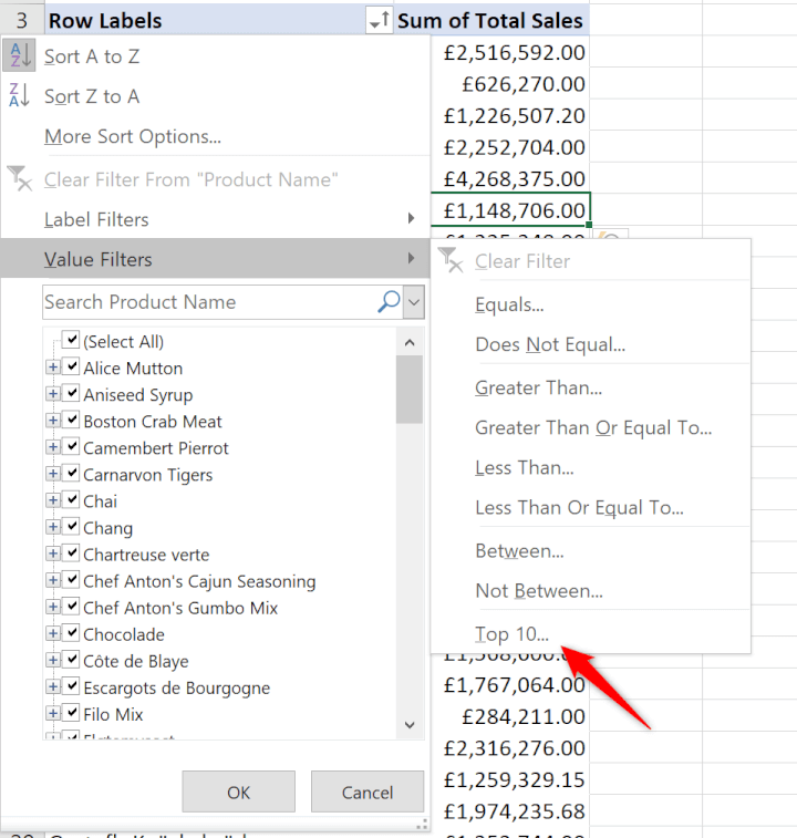
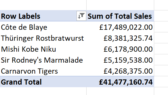
We would like to import these 3 files into an Excel workbook to analyze them and find the top 5 selling products, as well as which countries we received over £10 million.

Previously we would have imported the files into three different sheets and then used VLOOKUPs to pull the data into one big list for use in a PivotTable.

But with Power Pivot, we will import them directly into the data model for efficient storage. Then create relationships between the tables (instead of thousands of VLOOKUPs). And perform analysis with a PivotTable and DAX.

How to get and install the Power Pivot add-in

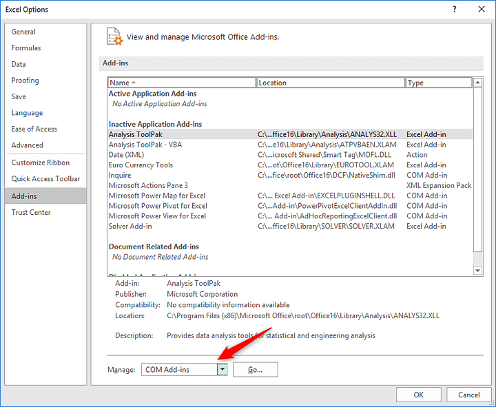
In Excel 2013, 2016 and 365 Power Pivot is included as part of the native Excel experience. It will just take a few seconds to install it from the COM add-ins the first time you want to use it.

Click File > Options > Add Ins.

Select COM Add-Ins from the Manage list, and click Go.

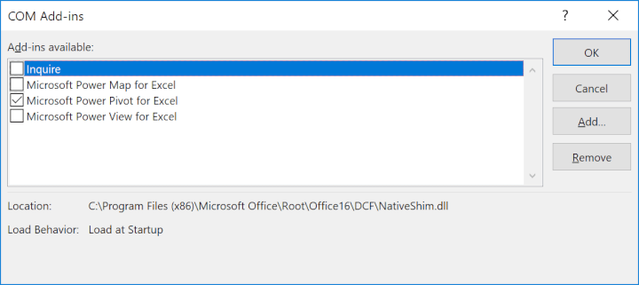
Check the box for Microsoft Power Pivot for Excel and click Ok.

The Power Pivot tab will then be visible on the Ribbon.

If you are using Excel 2010 you will need to download the Power Pivot Add-In from the Microsoft Site.

How to import CSV files to the Data Model

We will now walk through our use case scenario.

You can download the files and follow along for some hands-on practice.

Firstly we need some data. This data could already be in Excel. But often if you are working with large data sets you are getting data from a database, a folder or multiple text/CSV files.

The best way to bring this data into Excel is by using Power Query. Power Query is a tool built into Excel to make importing and transforming external data simple.

Power Pivot can then be used to model and analyze this data. And it can all be refreshed with the click of a button in the future.

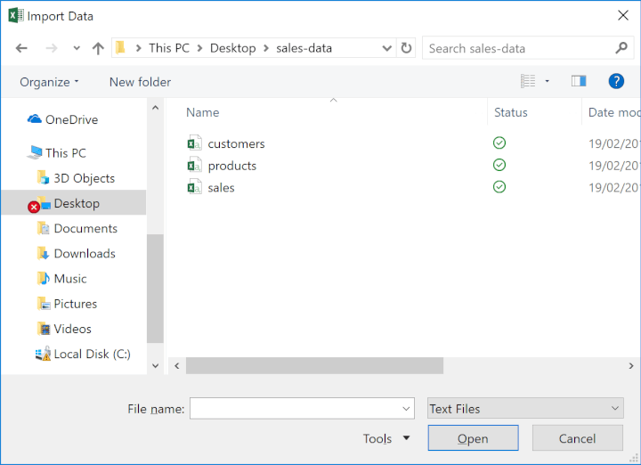
Power Query is outside the scope of this article, but here is a quick example of getting our sales data from CSV files. I will start with the sales.csv file.

Click Data > From Text/CSV

Locate the CSV file within the Import Data dialog and click Ok.

You will then see a window with a preview of your file. Click the Edit button at the bottom of the window.

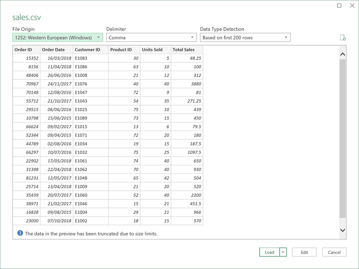
The Power Query Editor window will load. There are a lot of tools we can use here to transform the data.

This is just a quick example to get the data into the model for Power Pivot. So we will just close and load the data.

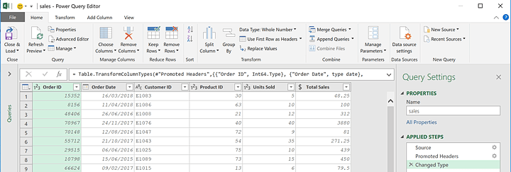
Click Home > Close & Load list arrow > Close & Load To

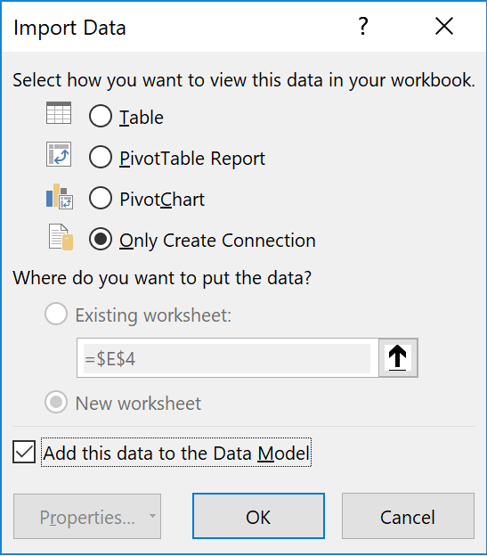
The Import Data window appears. Select Only Create Connection and check the box to Add this data to the Data Model.

The data is then loaded into the model. So you will not see it on the worksheet, but you will see a Queries and Connections pane appear showing the number of rows loaded.

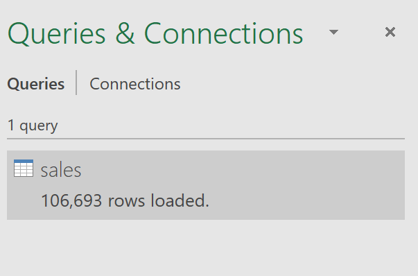
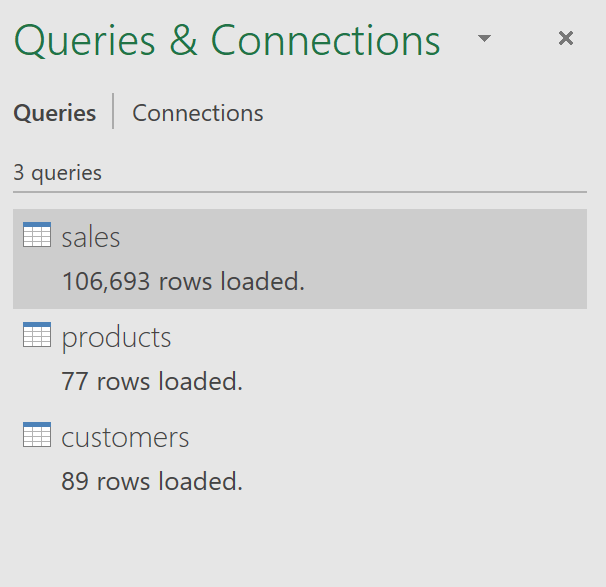
The image below shows the sales.csv file loaded. It contains 106,693 rows. That is a lot of rows, but you will see that it does not impact the performance of calculations in Power Pivot.

Repeat the process for the other 2 CSV files. When finished the loaded queries will look like below.

Viewing the Data Model in Power Pivot

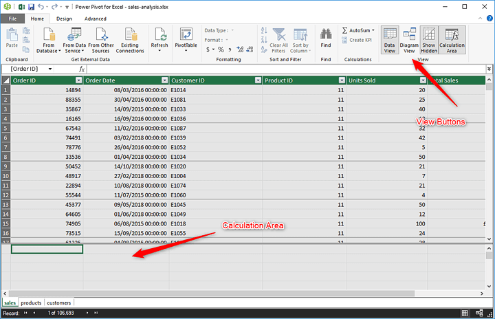
Let's have a look at how the data looks in Power Pivot. Click the Manage button on the Power Pivot tab.

The Power Pivot for Excel window is displayed.

The initial view you are taken to is called the Data View. The tables of data are shown on different tabs, similar to worksheets. This is, however, just a display and not how they are stored.

Underneath the tabs is the Calculation Area. We will talk more about this shortly when we cover measures.

 

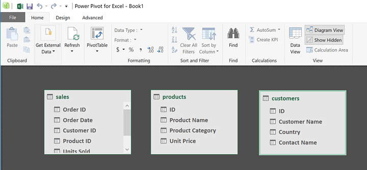
In addition to the Data View, there is also a Diagram View. You can jump to this by clicking the Diagram View button on the Home tab.

This provides a better view of the model and is great for viewing the relationships between the tables which we will create.

Create relationships between the tables

With the tables loaded into the model, we will now create relationships between them. This will enable us to create PivotTables using the data from all three tables.

The Diagram View is the easiest way to set this up. Let's start by arranging the window more efficiently.

Drag the Sales table under the Products and the Customers tables.

The Sales table contains the transactional information and is referred to as "the data", or "the fact table".

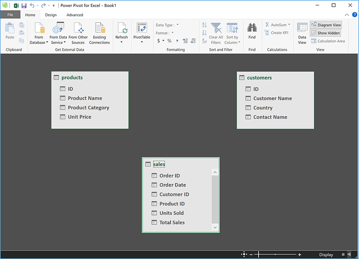
The Products table and the Customers table contain information on groups of objects that interact with the data and are referred to as "lookup", or "dimension tables".

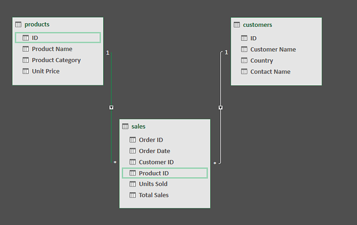
We will create two ‘one to many’ relationships. One between the Customers table and the Sales table, and another between the Products table and the Sales table.

This is because a customer could make one or many sales with us. And the same for the products. A product could be sold once or many times.

To create the relationship between tables we will click and drag between the Customer ID field in the Sales table to the ID field in the Customers table.

Repeat the step to create a relationship between the Product ID field in the Sales table and the ID field in the Products table.

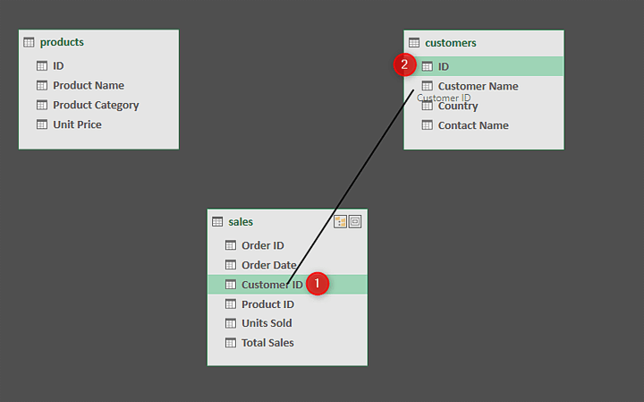
The image below shows the completed relationships. The filter direction of the data is displayed by an arrow, and a 1 and asterisk (*) symbols are also displayed to show the relationship type.

Create a PivotTable from the Data Model

With the Data Model set up, we can create a PivotTable.

Click Insert > PivotTable.

Excel automatically detects the Data Model and suggests creating a PivotTable from it. Specify whether you want the PivotTable on a new or existing sheet and click Ok.

The PivotTable appears and in the field list you can see the three tables. We can now access the fields from each table and drag them to the areas of a PivotTable as normal.

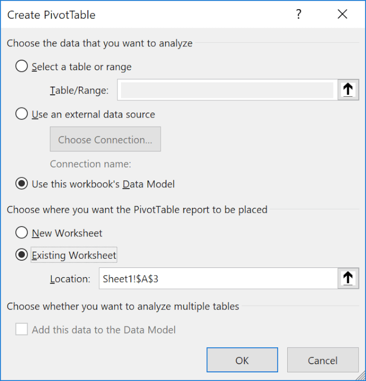
So what is Power Pivot? It is a PivotTable that uses data from the internal model.

Now let’s create one of our use case examples. We will find the top 5 selling products.

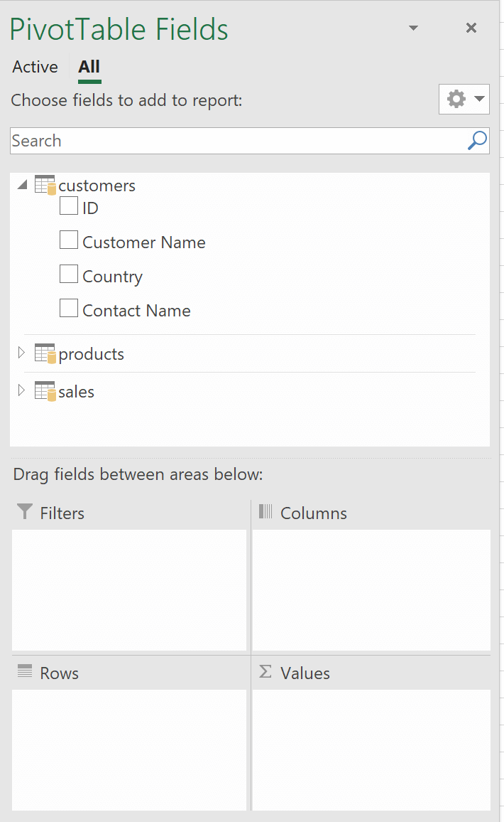
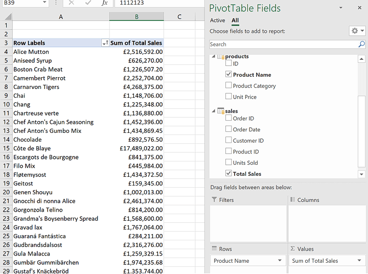
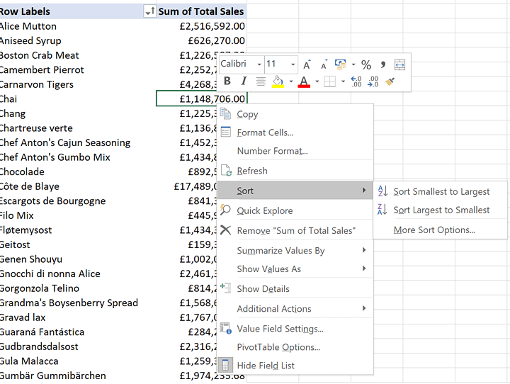
Drag the Product Name field from the Products table into the Rows area. Then drag the Total Sales field from the Sales table into the Values area.

This will sum the total for each product in our data.

We can then sort the list largest to smallest by the sales total. Right-click a cell containing a sales total and select Sort > Largest to Smallest.

Then we will filter the list to display only the top 5 products. Click the filter arrow for row labels, select Value Filters > Top 10.

Change the 10 to a 5 and click Ok.

We have the top 5 products in a PivotTable.

Now when we dragged the Total Sales field into the Values area of our PivotTable, it created what is called an Implicit Measure.

We can use a PivotTable from the Data Model in the same way as we may be used to doing. This is great at the beginning or if you’re just performing simple analysis. But it is better and more efficient to create measures and to use them in PivotTables.

Using DAX to create Measures

Let's begin to have a look at the DAX language to perform calculations in Power Pivot.

There are two types of DAX calculations - Calculated Columns and Measures.

A Calculated Column is used to create additional columns in your data model. And these columns can then be used as labels in the rows, columns and Slicer areas of a PivotTable.

It is encouraged to create these columns in the original data, or in Power Query instead of the model if possible. These columns can be really useful for a further breakdown of our data such as grouping dates into weekday and weekend labels.

In this article, we are going to create the other type of DAX calculation - called a Measure. Measures are calculations that are dragged into the values area of a PivotTable such as Sum and Average.

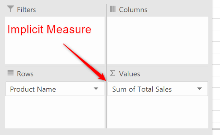
The DAX language is huge, going far beyond the standard Sum and Average. So creating these in the model provides far more power than within a standard PivotTable and Implicit Measures.

Measures created with DAX can also be used multiple times and in multiple PivotTables (but calculated just once). This improves the processing speed. You can also assign a format to a Measure so you won’t need to format them every time they are used.

We will create a Measure to sum the Total Sales field from the Sales table.

Click the Power Pivot tab > Measures > New Measure.

The Measure window appears.

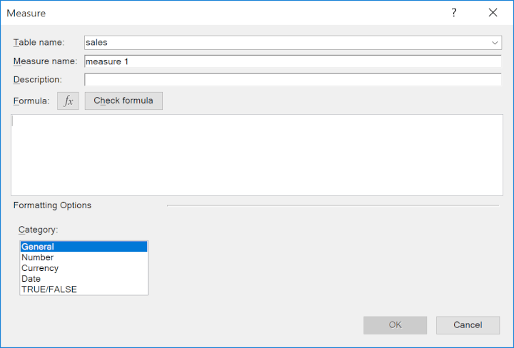
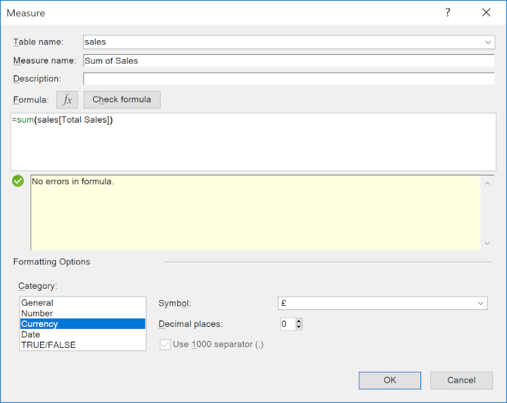
1. Select the table from the list that you would like the new measure stored within. This measure will be stored in the Sales table.
2. Enter a name for the measure. This measure is named Sum of Sales.
3. You can enter a description for a measure. Especially if complex. Here it is omitted since the name serves that role as well.
4. Enter the following formula into the box provided:  =SUM(Sales[Total Sales])
5. Click the Check Formula button. You will then receive confirmation that there are no errors in the formula.
6. Select a Currency from the formatting category. Then select the required currency symbol and how many decimals you would like to display. Click Ok.

Using a Measure in a PivotTable

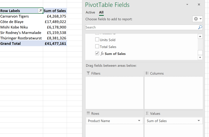
With the measure created we can use it in our PivotTables for analysis.

Using the PivotTable we created earlier in the tutorial, we can remove the Sum of Total sales implicit measure.

Our new measure is shown in the list of table fields and can be dragged into the Values area as a replacement.

We will now create our other use case of showing in which countries we received over £10 million and re-use the same measure.

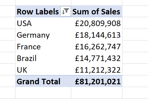
Insert a new PivotTable as before and drag the Country field from the Customers table into Rows, and the Sum of Sales measure from the Sales table into Values.

Sort the values largest to smallest and then click the filter button, Value Filters > Greater Than.

Enter 10000000 into the field and click Ok.

The countries that meet the criteria are shown as below.

Our measure has been used in both PivotTables to help us achieve both use cases. The DAX language is capable of far more and I encourage you to read further in that area.

In this article, we have answered the question of what is Power Pivot and demonstrated two business use cases on how to use PowerPivot through the entire process.

We imported the data into the model, created relationships and a measure, and then used them in PivotTables.

Power Pivot is one of the best improvements to how we use Excel. It is an extremely powerful tool and this article is an introduction to what it is capable of. I encourage you to learn and develop your Power Pivot skills even further.

Ready to become a certified Excel ninja?

Start learning for free with GoSkills courses

Start free trial