How to Use the Excel RIGHT Function

---

Excel has functions that allow you to grab just a piece of data from a text string and place it somewhere else. When the piece you want is at the end of that string, the Excel RIGHT function might be just the thing you need. 

Purpose

The RIGHT function in Excel extracts a specific number of characters from a text string, starting from the rightmost character. This function relies on the relative position of characters in a text string.

Return value

The value returned by the RIGHT function is the character or characters in the original text string which meet the conditions stated in the formula.

Syntax

The syntax of the RIGHT function is: 

RIGHT(text, [num_chars])

Arguments

The text argument is the text string from which you want to extract characters. This may be entered as a text string within double quotes inside the formula itself, or (more commonly) it could refer to a cell reference that contains the characters to be extracted.

The num_chars argument is optional. It tells Excel how many characters you want to be copied from the original text string, starting with the last (rightmost) character. If num_chars is omitted, it is assumed that you only want the very last character.

For example: 

=RIGHT(“apples and oranges”,7) will return the word oranges.

=RIGHT(“apples and oranges”) will return the letter s.

Remarks

• If num_chars is zero, RIGHT will return an empty cell.
• If num_chars is not an integer, Excel will truncate the number and return the relevant characters.
• If num_chars is a negative number, RIGHT will return a #VALUE! Error.

---

---

Using RIGHT to solve problems

Basic application

In its simplest application, RIGHT can be used to extract the last n characters from a cell, like in the example below.

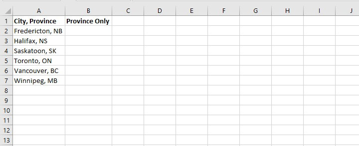To extract the last two letters in Column A to isolate the two-letter abbreviation for each province, the RIGHT function is the perfect solution.

=RIGHT(A2,2)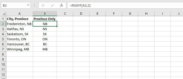

It hardly gets easier than that.

Using LEFT, MID, and RIGHT functions to split data of fixed length

RIGHT is sometimes used with the MID and LEFT functions to split values in one cell across several cells. As their names suggest, MID is used to extract characters from somewhere in the middle of a text string, and LEFT is used to grab leftmost values from the string.

We can use two or all of these functions when we want to break up a text string into separate pieces.

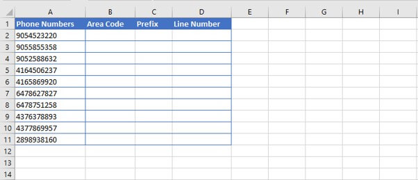
For example, the following dataset contains telephone numbers which we would like to split into three separate columns as follows:

• The area code, consisting of the first three numbers. 
• The prefix, consisting of the next three numbers. 
• The line number, consisting of the final four numbers. 

Step 1

We would use the LEFT function to grab the first three numbers. The syntax of the LEFT function is:

=LEFT(text, [num_chars])

• Text is the text string to be split.
• Num_chars is the number of characters in text to return, starting with the leftmost character. If omitted, only the leftmost character is returned.

=LEFT(A2,3)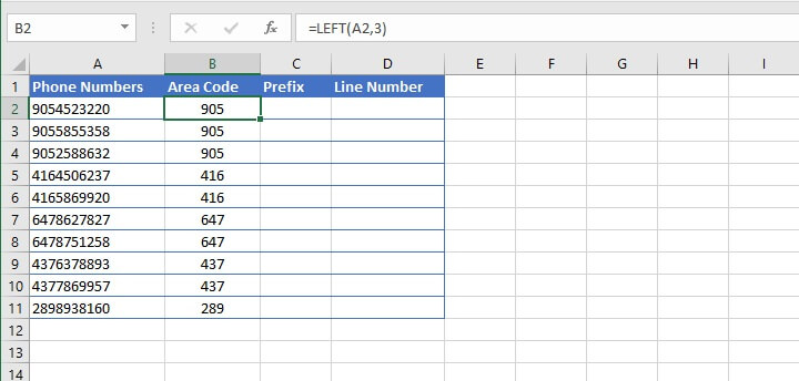

With the above formula, Excel extracts the three leftmost characters from the string in cell A2.

Step 2

Then we can use the MID function to get the next three numbers. The syntax of the MID function is:

=MID(text, start_num, num_chars)

• Text is the text string to be split.
• Start_num is the position number of the first character to be returned, counting from the leftmost character in text.
• Num_chars is the number of characters in text to return, starting with the leftmost character. 

All three arguments in the MID function are required.

=MID(A2,4,3)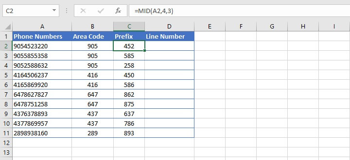

In the above formula, we are asking Excel to extract three characters from the string in cell A2, starting with the fourth character from the left.

Step 3

Finally, we use the RIGHT function to extract the last four numbers.

=RIGHT(A2,4)

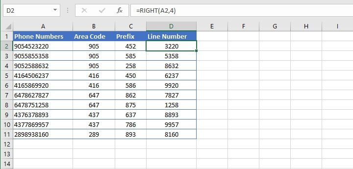Now we have successfully split the text in one cell into three cells using a formula. This is a great solution for text strings that are of fixed length.

Using RIGHT, LEN, and FIND to extract strings of variable length

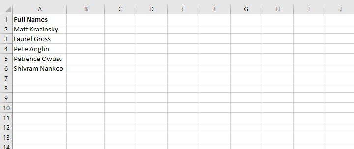
The problem is a little trickier when the values we want to extract are of variable lengths. If we want to get the last names from the following list, we wouldn’t be able to just use the RIGHT(text, [num_chars]) syntax because the last names aren’t consistent in length.

We can use the LEN and FIND functions to determine the length of the text string and to locate the position of the space character.

The syntax of the LEN function is simply:

LEN(text)

• Text is the cell reference or cell reference which contains the characters to be counted.

The syntax of the FIND function is:

FIND(find_text, within_text, [start_num])

• Find_text is the text you want to find.
• Within_text is the text string within which you want to search.
• Start_num (optional) is the position number of the character where you want to start searching. If start_num is omitted, FIND will start searching from the first character in the string.

We can use LEN and FIND to calculate the num_chars argument of the RIGHT function.

=RIGHT(A2,LEN(A2)-FIND(“ ”,A2))

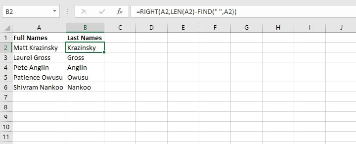The LEN function counts the number of characters in a text string, and FIND returns the position number of a character. The LEN(A2)-FIND(“ ”,A2) section of the formula above results in 14-5, telling us that the RIGHT formula will return the last 9 characters from the text string in cell A2.

We can copy the formula to the other rows for Excel to perform the same calculation and return the last names.

Note that the FIND function is case-sensitive. In this case, it doesn’t matter because we want to find a space character. But if you want to do an extraction using a non-case-sensitive character search, use the SEARCH function instead. 

Excel RIGHT function troubleshooting

There are a few times when you might not get the result you expected when using the RIGHT function. Here are some common problems.

1. Working with dates

Understanding that RIGHT is a text function is very important. This means it will convert all values to Text format. So trying to pull the year only from cell A1 below will not return a value of 2021. 

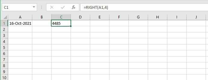The reason for this is that while we are seeing a display of 16-Oct-2021, Excel dates are really just numbers displayed in a way that makes sense to us. But for Excel, the date displayed as 16-Oct-2021 is stored as a number string. 

So when we ask Excel to use the RIGHT function to return the last four characters from that string, Excel returns 4485, the last four numbers which represent the string displayed to us as 16-Oct-2021.

The best (and simplest) solution for this problem is to use the YEAR function instead.

=YEAR(A1)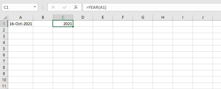

2. How to get a numeric output with RIGHT 

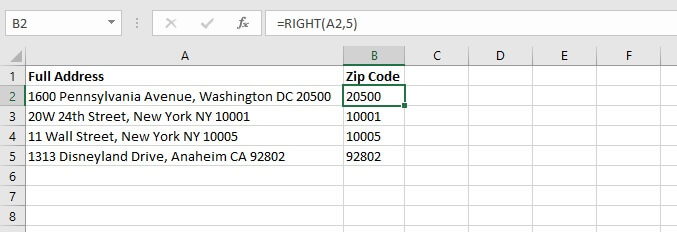
Understanding Text versus Number formats is also useful in a situation like the one below.

We can extract the last five characters from a text string to get the zip codes from an address. However, notice that the numbers are aligned to the left of the cell. This indicates that these values are stored as text instead of numbers.

If we want values that represent numbers to be stored in Number format, we can combine RIGHT with the VALUE function, which is specifically designed to convert a number that is stored as a text string to a number.

=VALUE(RIGHT(A2,5))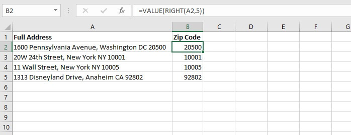

Now the zip codes are stored in Number format.

3. Fewer characters than expected

If you know how many characters make up your desired output, but your RIGHT formula only returns some of the characters, maybe there are extra spaces in your original text. 

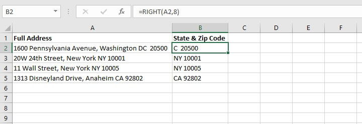The formulas in Column B were created to extract the two-letter state abbreviations and zip codes, but cell B2 returned only one character for the state. This is because there is an extra space between “DC” and “20500”. This sometimes happens when data is entered manually, and can easily be missed. 

We can fix this by combining RIGHT with the TRIM function. TRIM is designed to remove all spaces from a text string except for one space between words.

=RIGHT(TRIM(A2),8)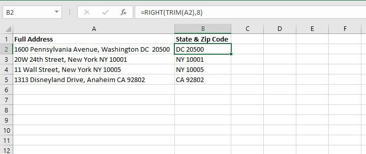

---

Quick note on combining functions: If you’re just learning how to nest (combine) functions, here’s a golden tip. Whatever action you want Excel to perform first should be in the inner parentheses. 

This is because since the result of those calculations will be needed for the other function(s), Excel wants to store that information in its memory for the subsequent actions.

That’s why for the situation above, we trimmed the full address first, then extracted the last eight characters. If we did it the other way around — TRIM(RIGHT(A2,8)) — the extra spacing would still be there. 

---

RIGHT vs. RIGHTB 

If you’re interested in learning about RIGHTB, you’ll want to know that the only difference between RIGHT and RIGHTB is that RIGHT returns the number of characters in a text string. RIGHTB returns the number of bytes used to represent the characters in a text string.

RIGHTB counts 2 bytes per character only when a double-byte character set (DBCS) language is set as the default language. The languages that support DBCS include Japanese, Chinese (Simplified), Chinese (Traditional), and Korean.

Otherwise, RIGHTB behaves the same as RIGHT, counting 1 byte per character. For this reason, we have only discussed RIGHT in this resource.

Sound off

Have you found any other uses for the RIGHT function? We’d love to hear about them. Leave a comment below!

You can also try our Excel Basic and Advanced course to continue boosting your Excel skills.

Ready to become a certified Excel ninja?

Start learning for free with GoSkills courses

Start free trial