11 Best Excel Tips for Beginners

Most people try to limit their Excel exposure to the bare minimum (and even actively avoid it like that one weird relative we all have). But whether it be a project at work or just a personal budget, you need to know basic Excel to get things done right and done quickly. To help you get the most out of Excel, we’ve put together a batch of the best Excel tips for beginners.

1. Adding frequent actions to quick access toolbar

Looking around any version of Excel you’ll notice there’s an endless array of tools at your fingertips. But most beginners use just a few of these repetitively. Instead of switching between the different tabs of the ribbon every time, you can add your personal favorites to what’s known as the Quick Access Toolbar.

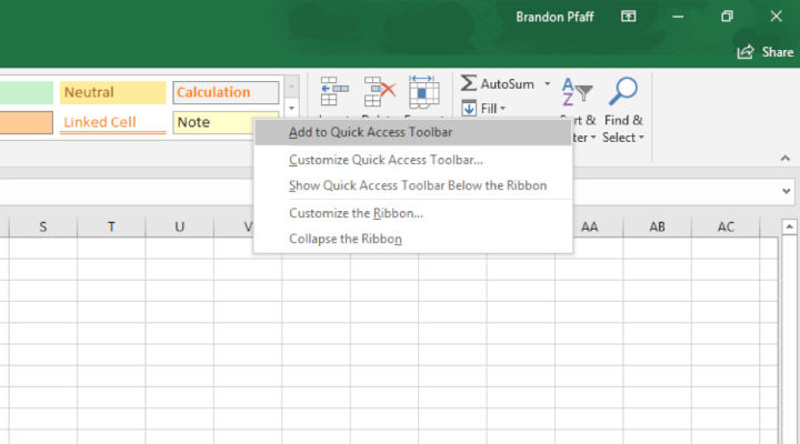
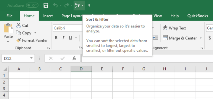
Microsoft offers several ways to make this happen but the easiest way is to right-click on what you want to add and select “Add to Quick Access Toolbar”. One of my personal favorites in my QAT is the Sort & Filter function as I usually work with a lot of data.

Before:

After:

Once you have your favorites added, you can also rearrange your QAT  shortcuts by right-clicking on it and then clicking “Customize Quick Access Toolbar...” in the menu. With your customized QAT you’ll be blazing through your next spreadsheet with ease.

2. Filtering data

Speaking of a lot of data, Microsoft has amazing tools to handle it all, which probably explains why it became the most important workplace computer program around the world.  Excel’s basic function for handling all this information is the Sort & Filter function. This is so useful because it allows you to rearrange and summarize data in a way that’s actually useful.

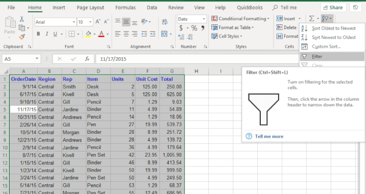
To do this, highlight all the data you want included in the filter (a quick way to do this is Ctrl + A). Then, click the funnel icon in the top left of the Home ribbon.

Now there will be a drop-down arrow at the top of each column in the filter. Here, you can select different values in the table and sort them. For example, let's say you wanted to see how many orders were made in a certain time frame. Just filter on the date column and select your desired time frame.

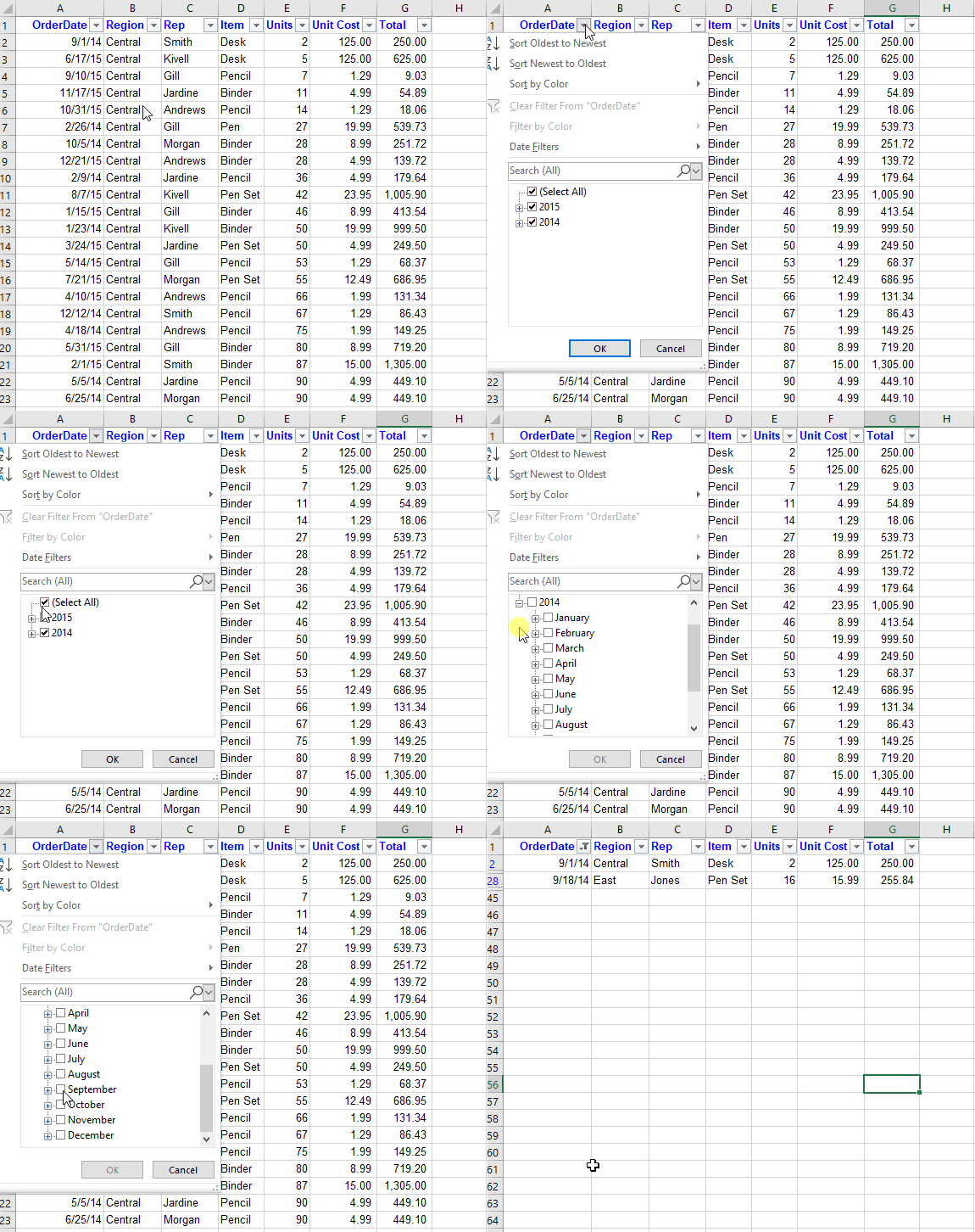
From our example, you can quickly see there were only two orders in September 2014.

3. Adding dynamic header/footers

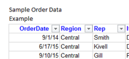
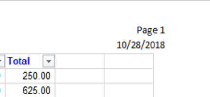
While it seems everything is going paperless, sometimes there’s still a need to print. One of the best ways to keep track of what's printed out of Excel is by adding page numbers, timestamps and file paths to the header or footer. To make sure you don’t have to update these values every time you need to print a spreadsheet, you can add formulas that update automatically.

First, change your view of Excel so you can see the header and footer.

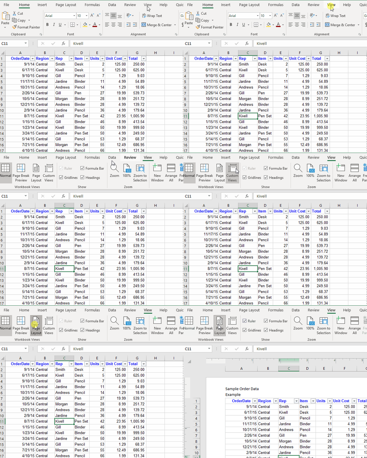
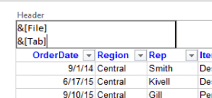
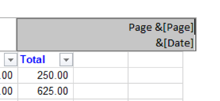
Next, add the following text to your header footer:

File name	&[File]
Sheet name	&[Tab]
Page number	&[Page]
Date	&[Date]

Before:

After:

4. Setting print areas on sheets

Now that you know how to automatically update what prints in the margin, another time-saving trick is set up print areas for your tabs to update what prints within the margins. If you like to keep all your work on one spreadsheet but only need to print out a certain portion, setting the print area is a great way to save time when you hit Ctrl + P.

To set your print area, highlight the cells you want printed. On the Page Layout ribbon, click the drop-down under Print Area and select Set Print Area.

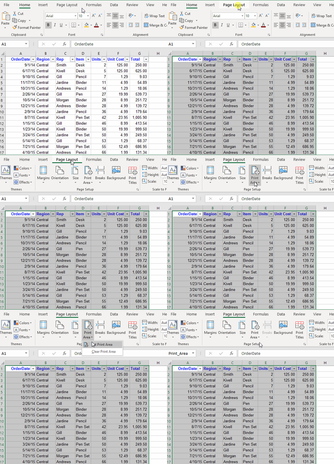
In the same drop-down menu, there’s the option to clear the print area. This is useful if you’ve changed your spreadsheet and want to add more to printable area.

5. Paste Special settings

There are so many different ways to accomplish tasks in Excel. Consider the simple copy and paste functions. As if Ctrl + C and Ctrl + V didn’t make copying easy enough, Microsoft built Paste Special.

Here’s how it works. Say you want to copy and paste something but not everything like a just a number or format. Instead of copying everything and removing what you don’t want, you can use Paste Special. To do this, copy your information as usual, but instead of using Ctrl + V, right click and select Paste Special from the menu.

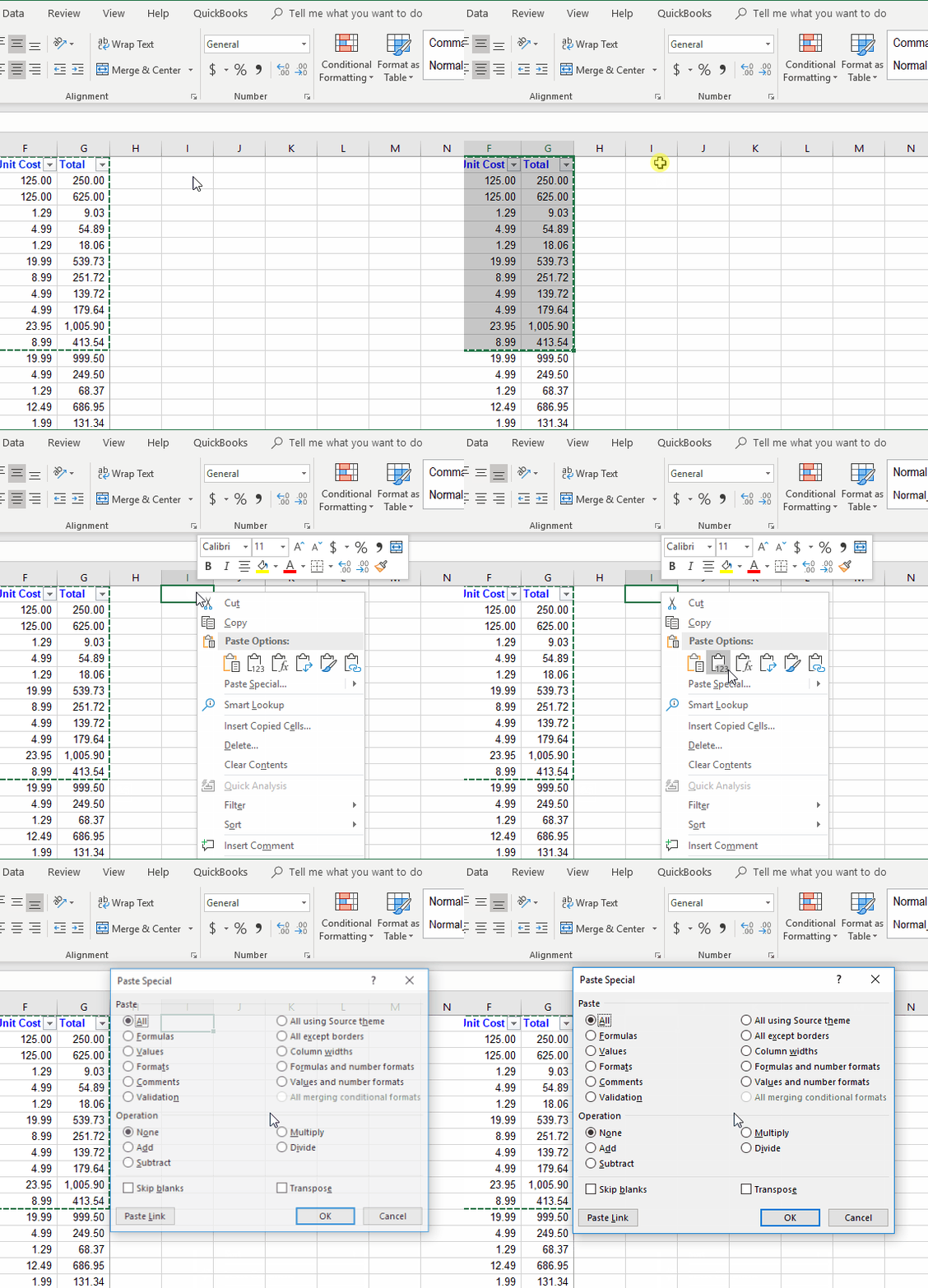
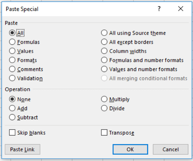
Some of the more popular Paste Special options include:

• Values - use this option if you only want to paste the text you see in the cells. It will leave all formatting unchanged.
• Formulas - Need to keep that formula but don’t need the formatting? Formulas allow you to do just that.
• Formats - Use this option to duplicate formats while leaving existing values and formulas.
• Column Widths - For when all your columns need to be a uniform width, this option saves a ton of time instead of adjusting them manually.

6. Group/ungroup columns to hide detail data

Spreadsheets with a bunch of complicated and detailed information can be hard to read and analyze. Luckily, Excel provides an easy way to collapse and expand the messy details to create a more compact and legible view.

Grouping in Excel works best for structured worksheets that have column headings, no blank rows or columns, and data is sorted by at least one column.

Select all the data you want to summarize in the group. Then, go to the Data tab > Subtotal. This will bring up a pop-up in which you can select how the data should be grouped and summarized. In the example below, we grouped by the change in OrderYear and summed on Total. This will show us total sales for each year and in total.

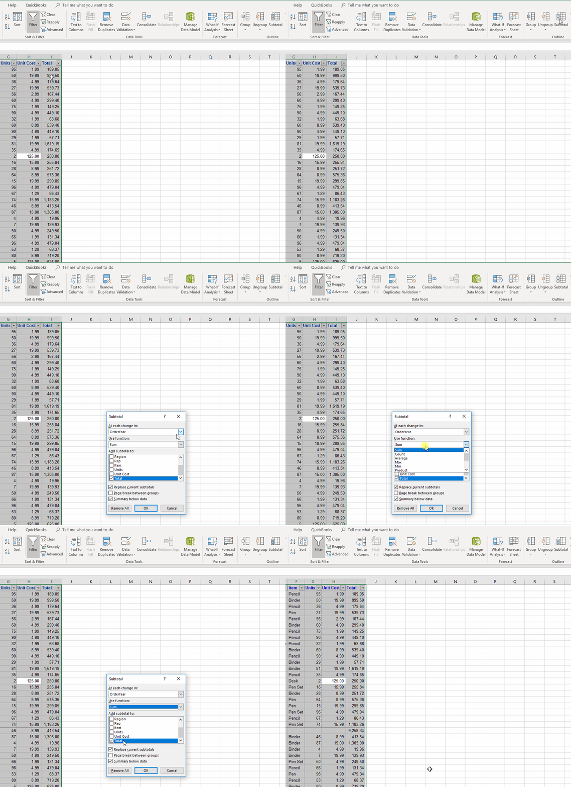Here is the result:

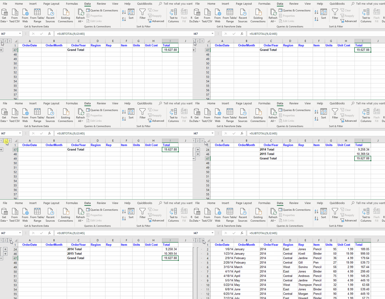
Now with just a few clicks, you can go from meaningful summaries to fine detail on the same spreadsheet.

7. Protect sheets and workbook

When it comes time to send your Excel spreadsheet, it's important to protect the data that you're sharing. You might want to share your data, but that doesn't mean it should be changed by someone else. Luckily, Excel has built-in features to protect your spreadsheets.

To protect a sheet, click on the Review tab in the ribbon then Protect Sheet. This will bring up a pop-up box where you’ll add the unlock password and what functions users can still perform while the sheet is protected.

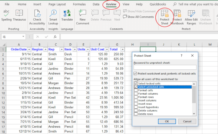
Once you click Ok, you are prompted to confirm the password and save the workbook. Now, if anyone tries to alter the information they will need that password. If you have a bunch of sheets you want protected, click on Protect Workbook follow the same procedure.

9. Trace precedent/dependent formulas

Have you ever used a worksheet that someone else set up? If you need to update the formulas and functions but do not know what other calculations will be affected you can spend a lot of time clicking around in the workbook with nothing to show for. Or you’re looking for a miscalculation and need to see where the data is flowing from.

Excel offers a simple way to review which cells are dependent upon others with Trace Precedents, and which cells contribute to others using Trace Dependents.

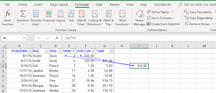
Both functions only work on the active cell selected so, unfortunately, it's one cell at a time. Click the Trace Precedents or Trace Dependents button in the Formula Auditing group of the Formulas tab to generate the blue arrows. Data flow follows the direction of the arrow with the blue dot being the precedent and the arrow being the dependent.

Below, Trace Dependents for cell E2 shows it only flows to cell G2.

And Trace Precedents for cell I4 shows cells E2 and F2 are the only cells flowing to it.

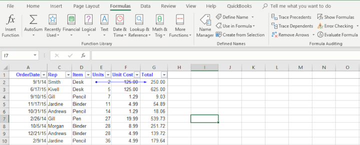
These functions work across tabs of the same workbook and different workbooks with one exception. Trace Dependents won’t work for external links for workbooks unless they are open.

9. Data validation for drop-down menus in cells

Using the drop-down list is a great way to impress your co-workers and boss with your Excel skills. At the same time, it’s a very user-friendly way to make sure custom Excel sheets function properly.

This tool is used to enter data in a spreadsheet from a predefined list of criteria. The main purpose of using drop-down lists in Excel is to limit the number of choices available for the user. Apart from that, a dropdown prevents spelling mistakes and makes data input faster.

This also gives you the possibility of controlling exactly what can be entered into a cell. This makes it perfect at validating inputs. First Select Data on the Ribbon and the Data Validation.

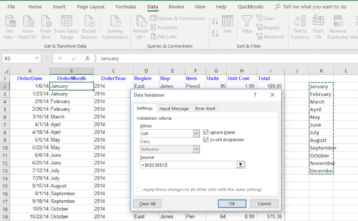
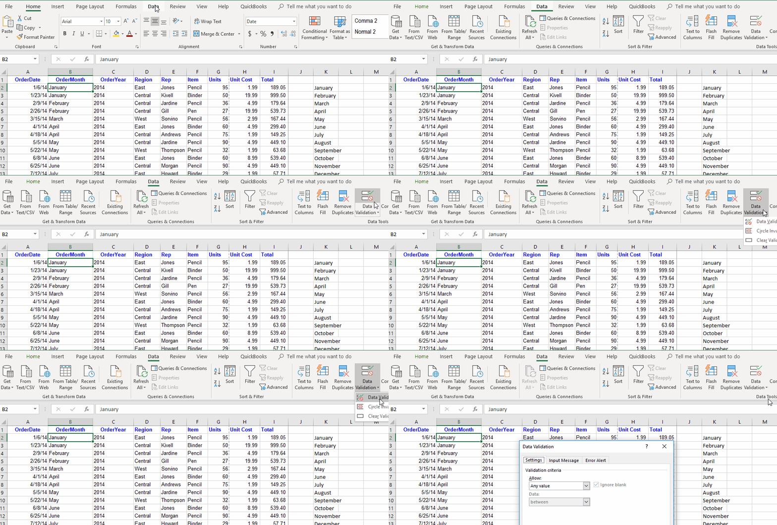Next, select your parameters. Below we used the months of the year to populate OrderMonth.

Once you click Ok, click on the drop-down arrow next to the cell and select from the list.

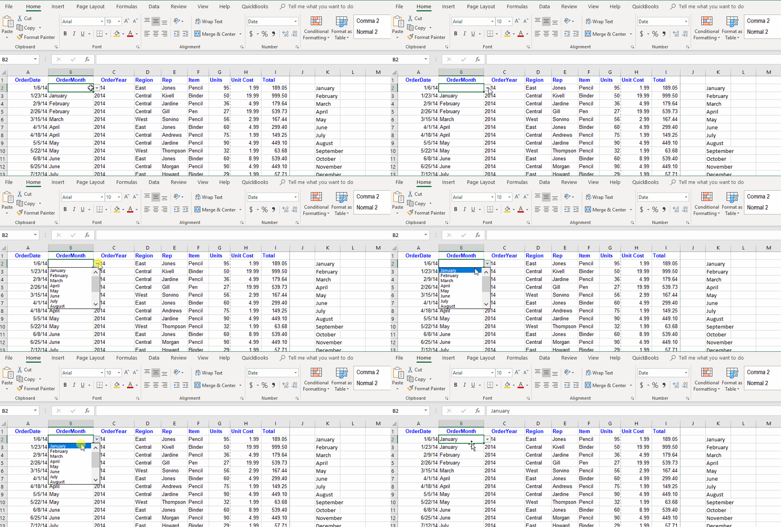
Note: now that one cell is set up, it can be copy and pasted in the remaining cells below.

10. Text-to-column - splitting data in one cell to multiple cells

Have you seen data in excel that you need but there’s other information in those cells that won’t work with your formulas? While there are some complex formulas that will help you split your text into new columns, it can consume a lot of valuable time. The speedy way to split this up is Text to Columns which splits all the selected cells at exactly the same point and puts the results in separate columns.

You can use Text to Columns in two different modes: fixed-width and delimited. Fixed-width is useful if can separate your data using a straight line through all the rows while delimited splits the text based upon the text such as every comma, tab, or space.

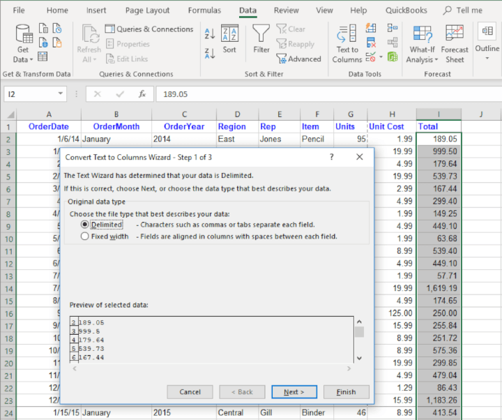
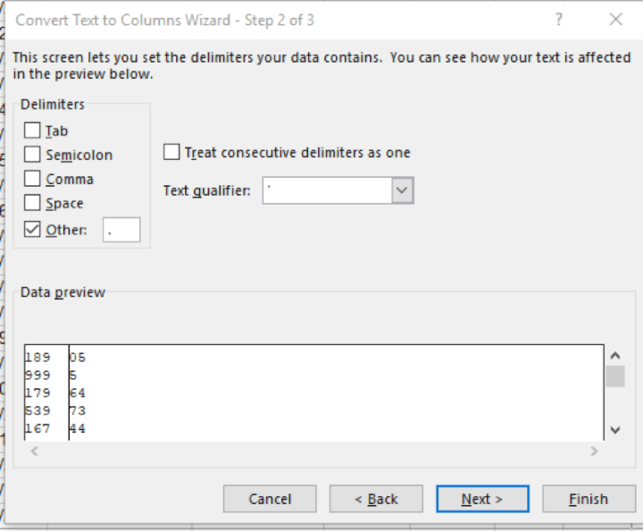
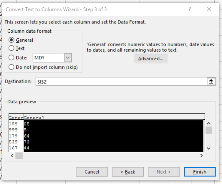
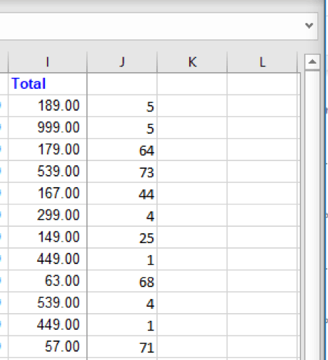
For example, let’s look at a delimited Text to Columns to remove cents from our total column.

Like most functions on the Data Ribbon, first, highlight your data and then click Text to Columns. Once here you’ll choose between fixed-width or delimited.

On the next screen, set your splitting criteria. In our example, we used the period.

On the final screen, you have the option to exclude sections and change the formatting. This will save you crucial steps later. Then click Finish.

And finally the results! All of the cents were placed in the column just to the right.

11. Creating simple graphs

One of the best ways to improve your Excel skills is being able to communicate your results to others. Graphics, images, and charts are great ways to visualize and represent your data to end users, and Excel does a great job of automating this process. Let’s take a look at how to set up a simple chart using our sample sales data.

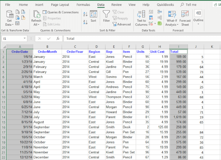
A simple graph starts with two sets of data, your independent (date) and dependent (results) variables. Below we have selected OrderDate and Total.

Clicking on Insert in the Ribbon you’ll see all the graphing options. For this example, a simple line graph will show us the total sales for each date.

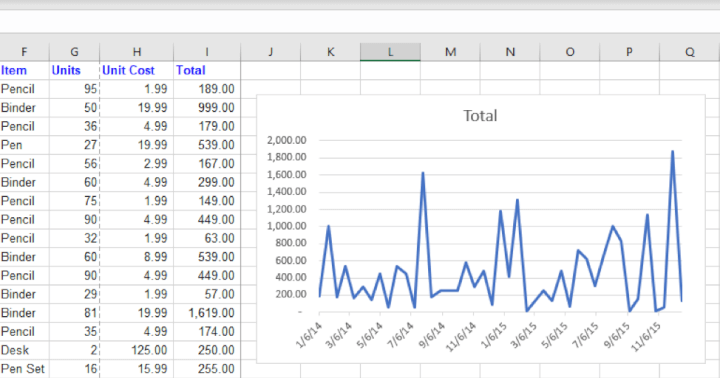
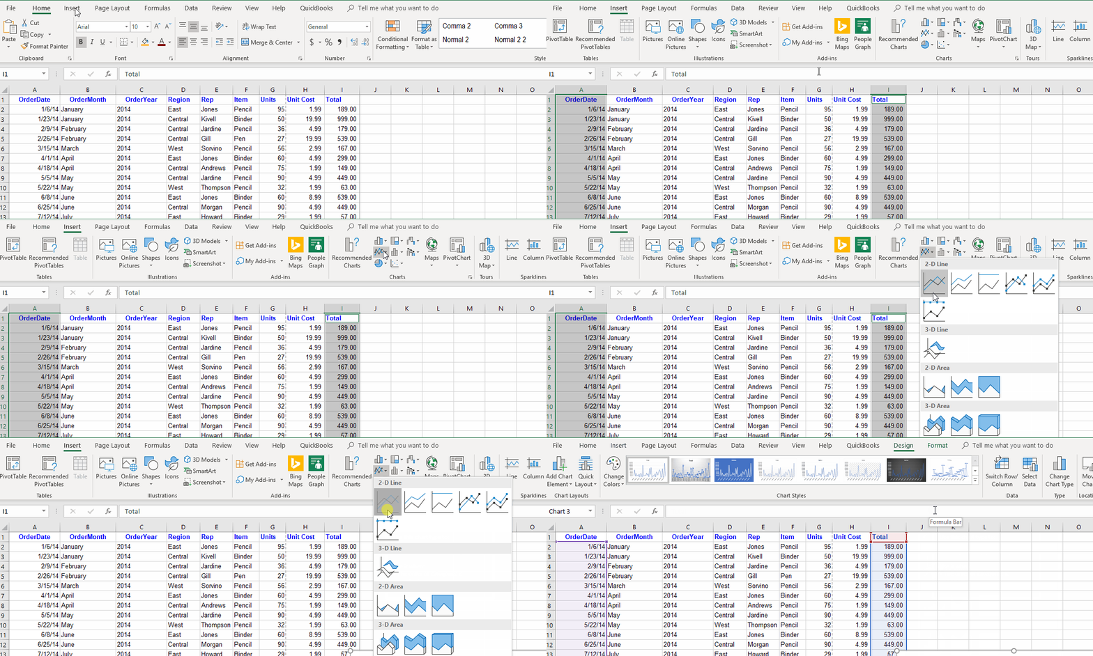Excel makes graphing so simple the results even include the title! So the next time you’re called into a last minute meeting you can create a simple graph on the fly in the meeting.

Bonus: Check out this lesson on how to create charts in Excel:

Conclusion

Now that you’ve learned more about Excel it's time to put that knowledge into action. These helpful tricks will make your work so much faster you’ll wish you knew about them so much sooner.

For more helpful Excel tips for beginners, check out our articles on the best Excel hacks, Excel essentials, and the best Excel shortcuts. You can even take our free crash course to quickly cover some Excel basics.

Want to improve your Excel skills even more? Don’t be the last person in your office to learn Excel - sign up for the comprehensive GoSkills Basic Excel course today!

Ready to start learning? Become an Excel ninja today with GoSkills

Level up your Excel skills

Become a certified Excel ninja with GoSkills bite-sized courses

Start free trial