How to Multiply in Excel

---

Arithmetic operations in Excel are really easy to do, and in some ways, intuitive. Take, for instance, multiplication. There are two main ways to perform a multiplication task in Excel. One is to use the multiplication operator, or asterisk (*), and the other is to use the PRODUCT function. 

In this article, we’ll explore in detail how to multiply in Excel.

Multiply using the asterisk 

The asterisk is used basically the same way as the standard mathematical multiplication symbol. It’s placed between the numbers being multiplied. Of course, this is considered a formula, and in Excel, we start formulas with an equal sign. 

---

---

Multiply explicit values

The quickest way to multiply 3 by 5 is to just type:

=3*5

When you hit enter, the product of the two numbers is displayed in the cell, but you can still view the formula that was entered by looking at the Formula Bar when that cell is the active cell.

This principle holds true when multiplying several numbers.

=3*5*6

Multiply using cell references

There may be other times when you have data in a cell and you want to make reference to that data when performing a multiplication operation. 

Below, the cost of each crate of produce can be calculated by multiplying the price per kilogram by the number of kilograms in each crate. 

We would substitute cell references for each value, either by typing in the cell references using each cell’s unique name (column first, row next convention), or by clicking on each cell while maintaining the format of Excel formulas. The price for one kilogram of apples is shown in cell B2, and the number of kilograms in a crate of apples is located in cell C2.

=B2*C2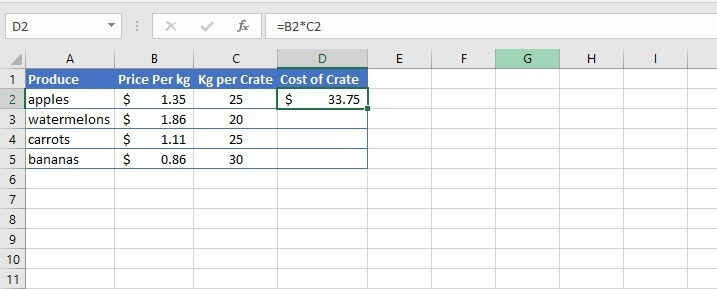

The formula is entered in cell D2, which then displays the product of the values in the two cells.

Multiply cell references by a constant number

Using an explicit value

The above principle can also be used to multiply cells in a column or row by a constant number.

=B2*100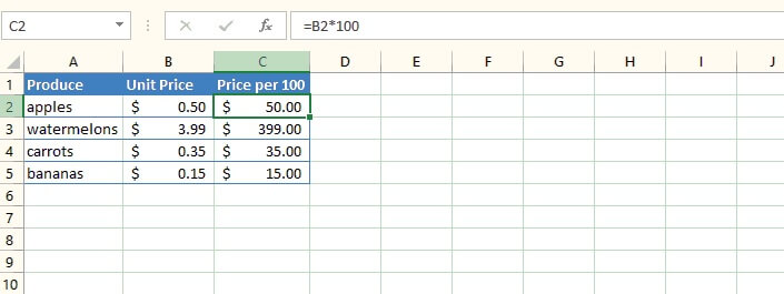

The same copying action is used to multiply each value in column B by 100.

Using absolute cell referencing

Sometimes it’s advantageous to enter the constant value in a single cell, and anchor that cell reference by using absolute cell referencing.

=B2*$C$1

By entering the constant in cell C1 and then placing dollar signs before the column and row numbers in the cell C2 formula, the reference to cell C1 will not be changed if the formula is copied to any other cell.

This way, there is only one step needed if an adjustment to that value needs to be made in the future. If we change the value in C1 to 50, then voila! All the cells referencing multiplication by cell C1 will be updated to multiply by 50.

Multiply by a percentage

We can find the percentage of a value by multiplying either the explicit value or cell reference by either the percentage or its equivalent decimal.

=33.75*8%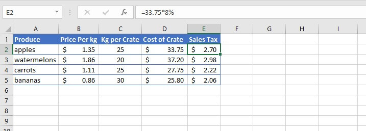

or

=D2*0.08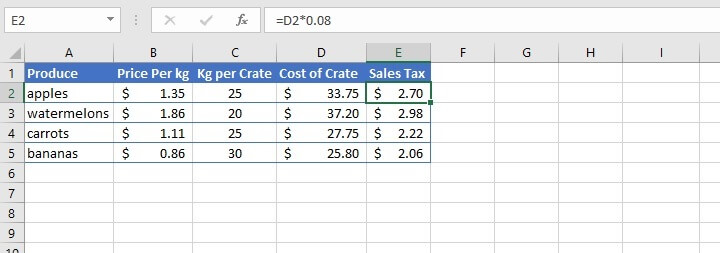

Multiply one column by another

Method 1 - Manually

Formulas can be replicated in the cells below by dragging the fill handle to copy the formula in cell D2 to cells D3 to D5.

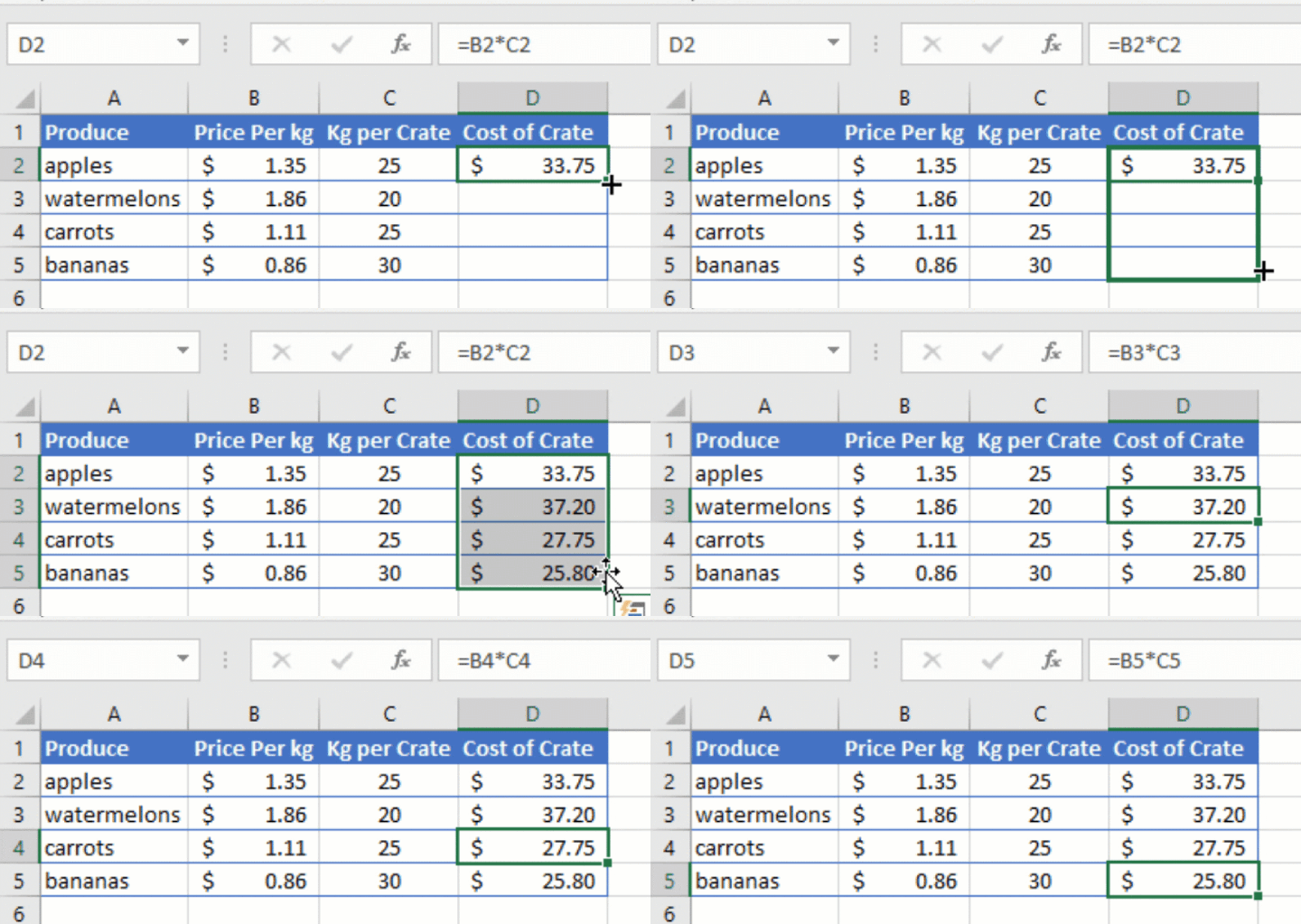In the example above, the value in each row will be multiplied by the value in the corresponding column. This action copies the relative formula and not the values themselves, because references in Excel are relative by default.

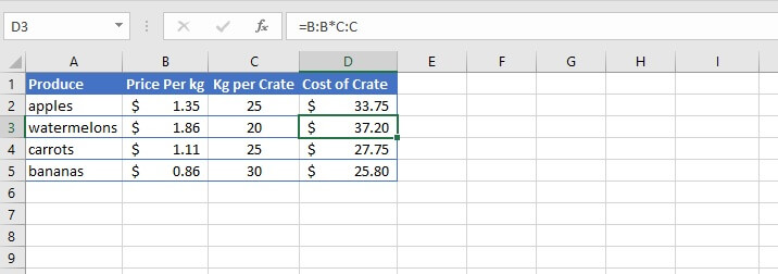
To multiply the contents of an entire column by another one, you could also enter:

=B:B*C:C

Then copy the formula downward as previously shown.

Method 2 - Using an array formula

An alternative way to multiply values in one column by another is to use an array formula (also known as a CSE formula). 

1. Highlight all the cells in your desired output location.
2. Identify the ranges that you would like to multiply.
3. With your output cells still highlighted, type your multiplication formula, for example:

=D2:D5*E2:E5

Do not hit ‘Enter’!

4. Press Control + Shift + Enter (hence, “CSE”) simultaneously on your keyboard. If you’re using a Mac, press Command + Shift + Enter instead.
5. The CSE formula multiplies each value in the first column by its corresponding value in the next column. The results are returned in the respective output cells.

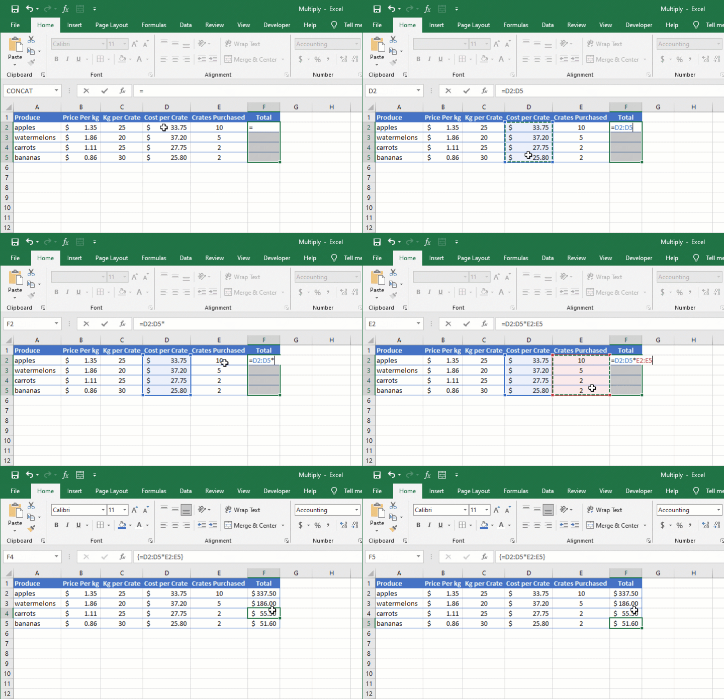
• You’ll notice that curly brackets appear around the formula in your Formula Bar. Excel does this to show that this formula was entered as an array formula.  If you type curly brackets around formulas yourself, it won’t do anything.
• In array formulas, only the cell where the formula was initially entered is editable. The other cells appear grayed-out.
• In all cases, the array arguments in a CSE formula must have the same dimensions. If not, Excel will return a #VALUE! error.

Multiply using the PRODUCT function

With the ease of using the asterisk symbol to perform multiplication tasks, you may wonder if having a PRODUCT function in Excel is worthwhile. Well, it is. Here’s why.

There may be times when you need to multiply several variables. If you imagine that a certain type of fruit tree produces two saplings each year, and that you start out with ten fruit trees, how many would you have at the end of three years?

One way to calculate this would be to multiply 10 by 2, by 2, by 2.

=10*2*2*2

Or using cell references in the worksheet below.

=A3*B3*C3*D3

The PRODUCT function performs this calculation by using arguments, separating each argument by a comma. An argument may be a value, a cell reference, or a cell range. In the example above, we can simply use a range since all the cells to be multiplied are contiguous, that is, together in a sequence.

=PRODUCT(A3:D3)

References to non-contiguous cells are separated by a comma. For example:

=PRODUCT(A3,C3:E3)

Note that the value in cell B3 is omitted from the calculation above.

SUMPRODUCT

Closely related to the PRODUCT function is SUMPRODUCT. The format (syntax) is similar in that the arguments are separated by commas. 

=SUMPRODUCT(array1, [array2], [array3],...)

The purpose of SUMPRODUCT is to multiply the values in the stated ranges, then return the sum of their products.

It replaces the longer three-step process shown below by eliminating steps 1 and 2.

1. Perform each multiplication operation. 
2. Copy the formula to each row as needed.

3. Find the sum of each product.

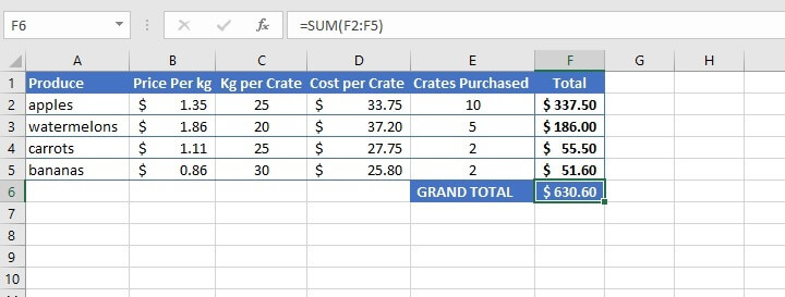On the other hand, with SUMPRODUCT, a single formula identifies each array, then does the multiplication and addition process simultaneously. A single value is returned, as shown below.

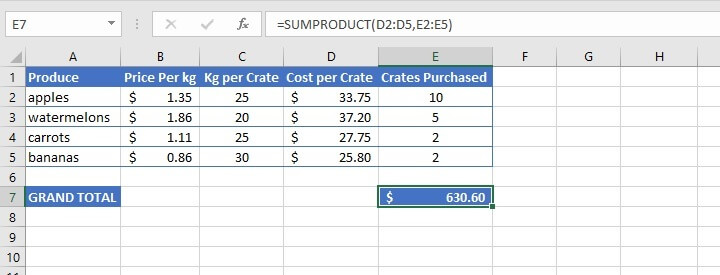If you only want to know the total without seeing the expanded values when the columns are multiplied by each other, SUMPRODUCT is the way to go.

---

Be sure to download the practice file so you can try all the above examples and get comfortable with how to multiply in Excel.

---

Learn more

Ready to be an Excel pro? 

You can start with this free Excel in an Hour course today, then take things to the next level with our other Excel courses, including the Microsoft Excel - Basic and Advanced course.

Free Excel crash course

Learn Excel essentials fast with this FREE course. Get your certificate today!

Start free course