Your Guide to VLOOKUP Table Array

It’s hard to maximize Excel’s features without knowing how to use VLOOKUP. This built-in formula performs a vertical search for a value located in the first column of a group of cells, and returns the value in the same row from a desired column. HLOOKUP uses a similar principle to do a horizontal search.

VLOOKUP has been the subject of tutorials, articles, and blog posts explaining how to use this powerful and game-changing tool. So why another VLOOKUP article? We're sharing some tips and best practices when using VLOOKUP, especially as it relates to table_array.

What is table array in Excel’s VLOOKUP?

Table_array is the second argument, or piece of information required, when inputting the VLOOKUP formula. Simply put, the table array argument refers to a group of cells which contains the source data and where you will be returning values from. Despite its name, the table array in VLOOKUP does not have to be an actual Excel Table.

A Table is a special object in Excel which behaves differently from an ordinary range of cells with data. Excel Tables have structured references, automatic formatting, and additional menu options along with a host of other features.

The term table array in a VLOOKUP formula, however, is used a little more loosely. A VLOOKUP table array is simply a dataset made up of at least two columns: the first column in the array is where we expect to find the lookup values, and at least one other column which carries the value we want to return in the output cell.

Syntax

The full syntax, or format, of the VLOOKUP function is:

=VLOOKUP(lookup_value,table_array,col_index_num,[range_lookup])

Lookup_value is the value you will be searching for.

Table_array is the range of cells where you will search for the lookup value. 

Col_index_num is the column number which contains the value you want returned. The column which potentially contains the lookup value must always be Column 1.

Range_lookup is a setting which tells Excel whether to accept a near match if the lookup_value is not in the first column of the table_array. TRUE accepts a near-match, and FALSE means only an exact match is accepted. Range_lookup is an optional argument, and if it is omitted, the default is TRUE.

How to use VLOOKUP

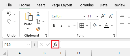
There are multiple ways to insert formulas in an Excel worksheet. If you are not yet experienced in doing this, you may find that the simplest way is to go to the output cell and click the Insert Function command just below the ribbon.

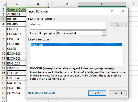
In the Insert Function dialog box, type VLOOKUP, press Go and click OK.

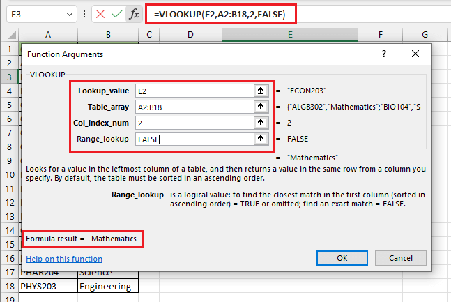
Enter the cell references in their respective fields using the Function Arguments dialog box.

To select the table array, enter the reference of the top left cell (the first cell) in the array range, colon, the bottom right cell (the last cell) in the array range. 

Alternatively, you can click and drag the range in the worksheet to select the table array when you get to the second argument in VLOOKUP.

In the col_index_num field, enter the column number of the values you want displayed in your output cell.

Notice that while the cell references or values are being entered in the Function Arguments dialog box, the formula is being displayed in the Formula Bar, and a preview of the result can be seen at the bottom of the window.

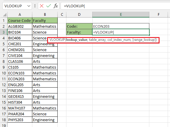
If you are already comfortable with building formulas without the Insert Function wizard, you can type it directly into the output cell.

Start with an equal sign and the function name, then follow the prompts to enter each argument.

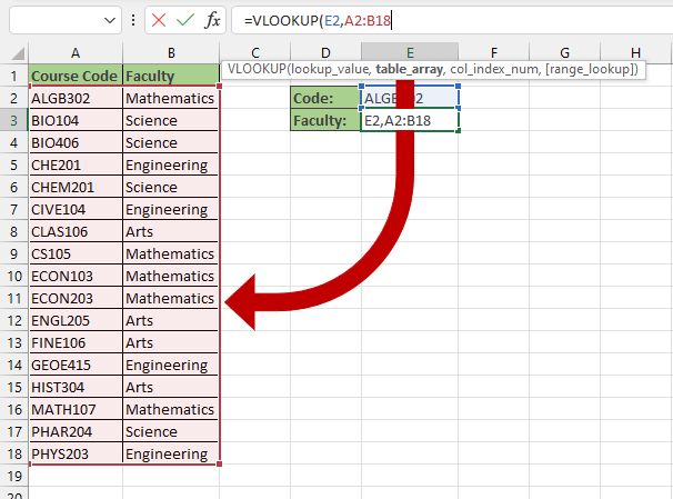
In the above example, the table array includes all the cells in the area A2:B18.

To finish off the formula, enter 2 as the col_index_num argument, and FALSE for range_lookup.

=VLOOKUP(E2,A2:B18,2,FALSE)

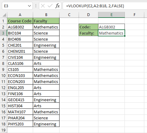
The formula looks up the value in cell E2 in the designated table array, and looks in the second column for the value in that same row. With this operation, the lookup value ALGB302 returns “Mathematics” from column 2 of the table array.

How to lock a VLOOKUP from a table array

Unless you make cell references in formulas absolute, Excel (by default) interprets them relative to the location of the cell in which they are entered. This means that when you copy formulas with relative cell references, the new formula is now pointing to a location that’s different from the original formula.

Of course, this is useful in cases like the one above, but in situations such as VLOOKUP, when we want to maintain the reference to the source data, we should ensure that the references for the table_array argument will not shift when they are copied. There are two options available for doing this.

1. Lock cell references

Making the cell references absolute will anchor, or lock them in place so that copying the formula will not point the references to someplace else on the worksheet. To anchor a cell reference, place a dollar sign before the reference to the column and a dollar sign before the reference to the row. An example is shown below.

=VLOOKUP($F$2,$A$:$C$18,2,FALSE)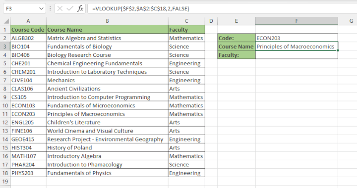

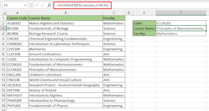
The cell references in the formula in cell F3 were locked because it makes copying the formula to cell F4 easier. (Note that in this example we also locked the reference to the lookup value cell, since copying the formula to the cell below would have also shifted the reference to cell F2 down by one row.) Once we’ve locked the cell references, we only need to adjust one element in the VLOOKUP formula - the column index number - so that the new formula will correctly display the name of the faculty.

=VLOOKUP($F$2,$A$2:$C$18,3,FALSE)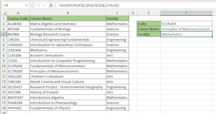

When locking cell references, you can manually type the dollar signs, or use the following keyboard shortcuts right after entering each cell reference: F4 (Windows), or Command+T (Mac).

2. Use named ranges

An alternative to using absolute cell references is to create named ranges. They accomplish the same thing, and as a plus, they usually make formulas easier to build and read. To create a named range:

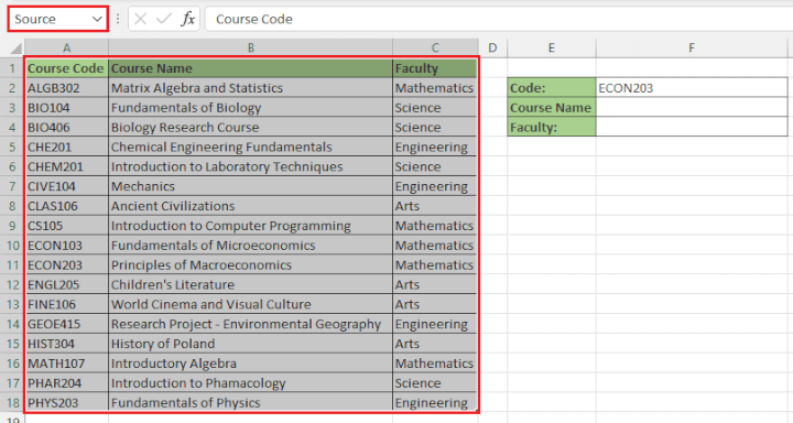
• Highlight a range that will be used frequently, in our case, the table array
• Enter a descriptive name for your range in the Name Box (e.g. Source).
• Press Enter.

In the background, Excel locks these references and associates them with the custom name you have created.

A maximum of 255 characters are allowed in user-defined Excel names, and spaces are not permitted. 

The great thing is that Named ranges are valid on all sheets throughout the workbook, so it is easy to do a VLOOKUP with a table array in another sheet without switching back and forth between sheets when formula-building.

Edit VLOOKUP table array

What if you made a mistake while entering the table array and your formula refers to the wrong source? This is an easy fix if the cell references were entered directly into the formula: just go into the output cell and correct the cell references in the second argument.

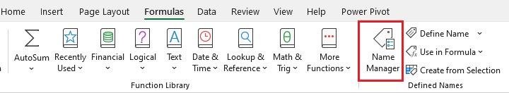
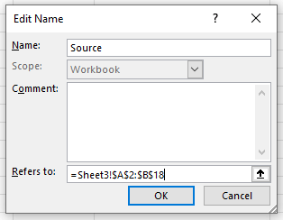
If you used a named range, go to the Formulas tab on the ribbon and click Name Manager.

In the Name Manager dialog box, ensure that the named range that you want to correct is highlighted, then click the Edit command. 

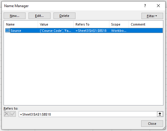
In the Edit Name dialog box, enter the correct cell references in the Refers To: field and click OK.

VLOOKUP not in the first column

Since VLOOKUP always assumes that the lookup value will be in the first column of the table array, how do you handle a situation like the one below?

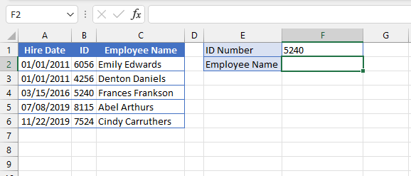
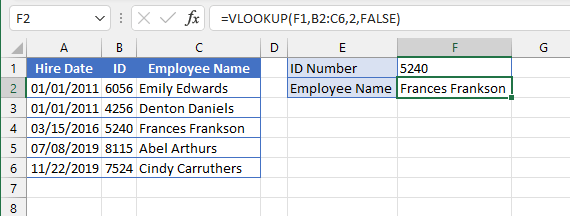
We want to use the ID number to return the employee name, but ID is actually the second column of the dataset on the worksheet. This case is not as problematic as it may seem. As long as the lookup column is to the left of the return column, VLOOKUP will work just fine. We simply need to define the table array beginning with the lookup column, ignoring column A since it is not relevant to our query..

=VLOOKUP(F1,B2:C6,2,FALSE)

VLOOKUP with multiple table arrays

You may need to do a more advanced lookup, one which requires Excel to look in multiple table arrays, perhaps even multiple sheets, for a value. This can be done by making use of a nested, or sequential, VLOOKUP formula.

 

The idea is to get Excel to look in one table array for a value. If it fails to find that value (an #N/A error result), we can point Excel to another table array by adding another VLOOKUP formula.

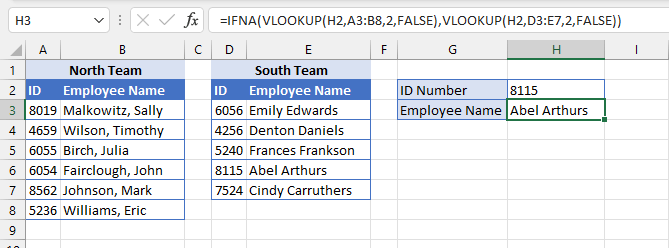
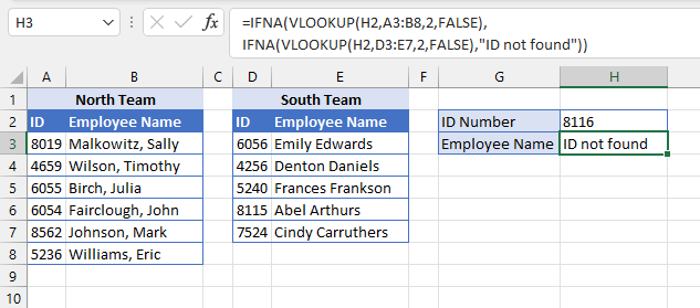
In the scenario below, we want VLOOKUP to search for the value in cell H2 by searching two different arrays - first, the array in cells A3 to B8, then the D3 to E7 array.

The IFNA function is preferred over IFERROR in this particular instance because it only looks for #NA errors, whereas IFERROR looks for all errors.

=IFNA(VLOOKUP(H2,A3:B8,2,FALSE),(VLOOKUP(H2,D3:E7,2,FALSE)))

The second VLOOKUP formula is nested withing the IFNA formula and becomes the value_if_error argument. 

Of course, we should also create a value_if_error if the second lookup also fails, by also nesting the second VLOOKUP with an IFNA formula.

=IFNA(VLOOKUP(H2,A3:B8,2,FALSE),IFNA(VLOOKUP(H2,D3:E7,2,FALSE),"ID Number not found"))

As many as 64 IF functions may be nested in a single Excel formula, and since VLOOKUP can be linked to data in another worksheet or even another open workbook, this makes its ability to use multiple table arrays quite powerful.

Table array with approximate match

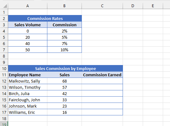
So far, all our examples have been with the exact match option. What if we wanted to accept an approximate match if no exact match is found? A scenario like this is shown below.

These sales reps are paid commission based on their weekly sales totals. This dataset has the lower limits for each commission percentage, that is, 0-19 sales will mean a 2% commission, 20-39 will be 5% commission, and so on.

In cells C12:C17 we need a formula that will look up the sales values in cells B12:B17 against the Commission Rates table and return the correct percentages.

For the optional range_lookup argument we would enter TRUE or just leave it blank, since approximate match is the default for VLOOKUP.

=VLOOKUP(B12,$A$4:$B$7,2)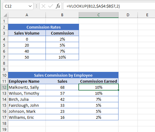

VLOOKUP completes the approximate match whereby if a lookup value is between two values in the table array, it chooses the smaller value and returns the corresponding value from the column index number. 

For VLOOKUP approximate value to work, the lookup values in the table array must be sorted in ascending order (smallest to largest).

Alternative to VLOOKUP

One of the biggest limitations of VLOOKUP is that the column index number cannot be to the left of the lookup values in the table array. This is not an issue with the XLOOKUP function though. If you have a current subscription to Excel 365, then you have access to XLOOKUP. You can also use Excel for the Web free to check out how to use this very flexible function.

Otherwise, there’s the old faithful INDEX MATCH function combo which allows you to bypass VLOOKUP’s constraints.
 

Ready to become a certified Excel ninja?

Start learning for free with GoSkills courses

Start free trial