Download the practice file for this video here - Click File > Download > Microsoft Excel.
This video covers the top six functions. Below we cover 20 Excel date functions.
Have you ever noticed that humans are incredibly obsessed with dates? Our level of happiness seems to be inseparably linked to an endless list of appointments, anniversaries, birthdays, holidays, workdays, and weekends. So why shouldn’t our most useful tools have systems for handling these dates of significance?
Managing dates in Excel requires special attention—they’re actually stored as serial numbers, but can be customized to give the appearance of text, or formatted based on local or personal preference.
There are more than 20 Excel date functions, all meant to simplify common operations involving dates.
Three things to know about Excel dates
- Dates in Excel are stored as unique serial numbers, with January 1, 1900 being considered Day 1. Each subsequent day is one day added to Day 1. Therefore January 2, 1900 is stored with serial number 2 and the following day is stored as 3 being the number of days since that date.
- Excel only recognizes dates on or after January 1, 1900. Special workarounds may have to be constructed to handle years between 1 and 1899.
- Changing the number format does not change the value of the number; it only changes the way that value is displayed.
Where to find date functions in Excel
The functions available to you will depend on the version of Excel you’re using. The quickest way to know what date functions are offered by your version of Excel is to click Formulas on the Excel ribbon and select the Date & Time dropdown menu from the Function Library.
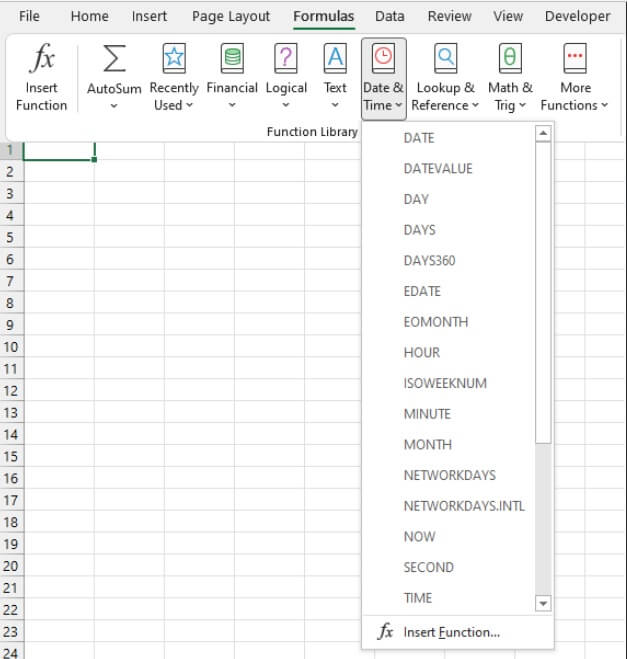 Let’s take a look at each date function, its purpose, and how to use it.
Table of contents
|
|
1. DATE
(Available in Excel 2007 and subsequent versions)
The DATE function is designed to eliminate confusion when working with dates in Excel.
Because dates can be written in a variety of formats, there can be misunderstandings when everyone isn’t on the same page. This can lead to problems when Excel does not recognize the numbers as dates and handles them in an unexpected way.
The DATE function establishes common ground by asking you to supply each element of your date in a particular order so that Excel assigns the correct date value to your input.
Syntax
The syntax of the DATE function is:
DATE(year, month, day)
All arguments are required.
- The year argument can be one to four digits representing the year. However, it’s recommended that all four digits be used for the year argument to avoid unexpected results. For example, an input of ‘07’ will be interpreted as the year 1907.
- Month is a positive or negative integer representing the month of the year.
- Day is a positive or negative integer representing the day of the month.
Important
- Excel only recognizes dates on or after January 1, 1900, therefore any year argument with a value between 1 and 1899 will be added to 1900. For example, a year of ‘1800’ will result in the year 3700, because 1800 was added to 1900.
- If the month argument is greater than 12, that number of months will be added to the first month of the year argument. For example, DATE(2000,18,1) will return June 1, 2001.
- If a negative value is entered for the month argument, that number of months will be subtracted from the first month of the year argument. For example, DATE(2000,-7,1) will return May 1, 1999.
- If the day argument is greater than the number of days in that month, that number of days will be added to the first day of the month argument. For example, DATE(1999,2,30) will return March 2, 1999.
- If a negative value is entered for the day argument, that number of days will be subtracted from the first day of the month argument. For example, DATE(1999,2,-7) will return January 24, 1999.
The way the date is displayed can be customized by using a built-in date format, or customizing your own.
=DATE(1999,1,24)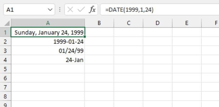 In all the above cells, the same formula was entered in all four cells but a different date format was applied to each cell by clicking on Date within the Format Cells dialog box.
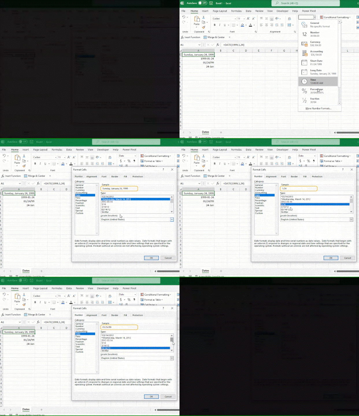 Alternatively, you can quickly call up the Format Cells dialog box by pressing the Ctrl+1 shortcut on your keyboard.
Get your FREE cheatsheet!
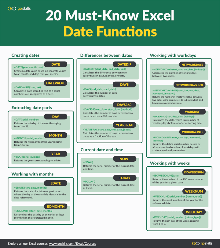
Download your printable cheatsheet with 20 Excel date functions here.
2. DATEDIF
(Available in Excel 2007 and subsequent versions)
The purpose of the DATEDIF is to calculate the difference in days, months, or years between two dates. This function is hidden and is not displayed in the Functions menu.
Syntax
Unlike other Excel functions, the syntax of the DATEDIF function does not appear as a tooltip when you type =DATEDIF. This means you’ll definitely need to know the format and how to use this function.
The syntax is:
DATEDIF(start_date, end_date, unit)All arguments are required.
- Start_date is usually the earlier of the two dates being compared.
- End_date is the later of the two dates being compared.
- Unit is the unit of time (whether days, months, or years) in which you want the results displayed. “Y” returns the number of complete years between the two dates. “M” returns the number of complete months between the two dates. “D” returns the number of days between the dates. The units must be entered within double quotes.
The image below shows an example of how to use DATEDIF in Excel.
 This function is especially useful for calculating ages. Note that the “years” unit will only calculate the number of complete years. To return a more precise age, consider using the YEARFRAC function instead.
A less common feature of DATEDIF is the ability to find the difference in days or months between two dates without taking the year into account. To do this, we would use the “YM” or “YD” units.
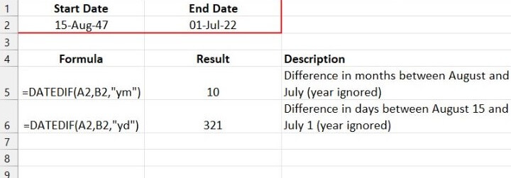 Note: Though there is an option to find the difference between the days in start_date and end_date by using the “MD” option for the unit argument, this results in a known issue so its use is strongly discouraged by Microsoft.
3. DATEVALUE
(Available in Excel 2007 and subsequent versions)
The DATEVALUE function converts a date formatted as text to a date serial number.
Syntax
DATEVALUE carries a single argument.
DATEVALUE(date_text)Date_text is a text string in one of Excel date formats. Date_text is entered within double quotation marks if explicit values are used, for example, DATEVALUE(“12/12/1999”). If date_text is a cell reference, no double quotes are used.
=DATEVALUE(“12/12/1999”)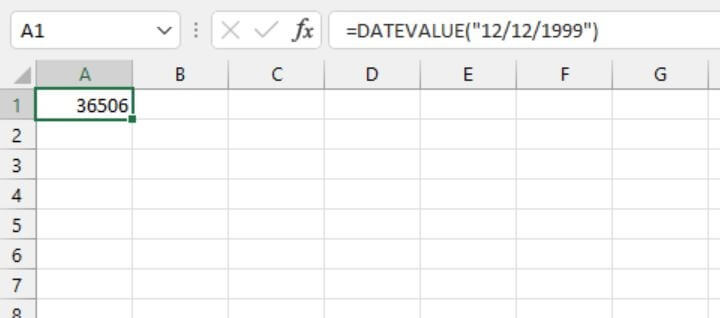 The value returned is the serial number used in Excel to store the date December 12, 1999.
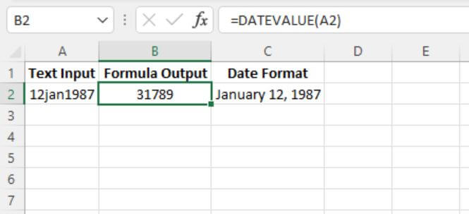 By default, Excel uses your computer’s regional settings to determine date formats. If it does not recognize the input as a valid date, DATEVALUE will return a #VALUE! error.
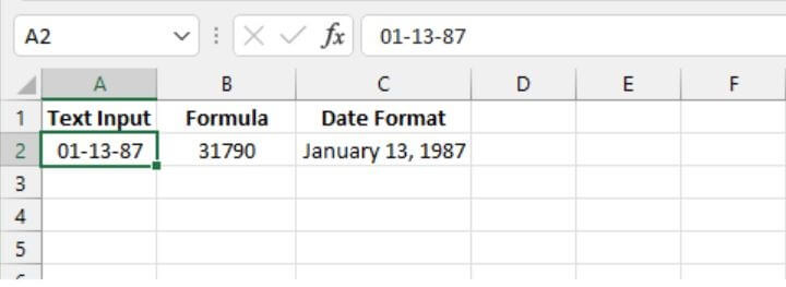
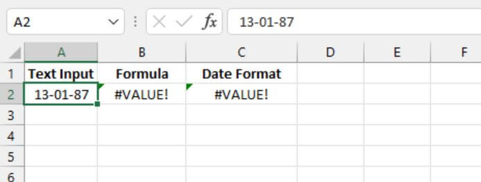 On a computer that carries a country date setting of month/day/year, a date value of 13-01-87 is interpreted as an invalid date, for which DATEVALUE returns an error. To correct this, you should either adjust your computer’s regional settings or change the text input.
4. DAY
(Available in Excel 2007 and subsequent versions)
The DAY function returns the nth day of the month ranging from 1 to 31. This can be useful for isolating the day element of a date.
Syntax
The syntax of the DAY function is:
DAY(serial_number)Serial_number is the Excel-assigned number of the date you want to query. The serial number is usually obtained as the result of another Excel function, such as TODAY, DATE, DATEVALUE, etc.
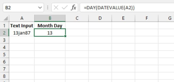 The number format of the output cell can be customized to display the day of the week.
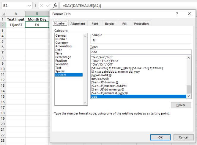 The custom format ‘ddd’ above converts the number to the three-letter abbreviation of day of the week represented by the given serial number. The format ‘dddd’ will return the full name of the day of the week.
5. DAYS
(Available in Excel 2013 and subsequent versions)
The DAYS function calculates the number of days between two dates.
Syntax
The syntax is:
DAYS(end_date, start_date)
- End_date is one of the two dates being compared.
- Start_date is one of the two dates being compared.
Excel returns the difference in the number of days by using the assigned date serial numbers.
The arguments for the DAYS function may be entered as a reference to cells containing the dates.
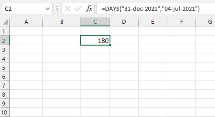
=DAYS(A2,A1)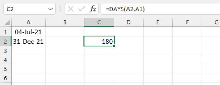 Alternatively, the arguments may be explicit dates entered as a text string:
 Note that if the end_date is earlier than the start_date, DAYS returns a negative value.
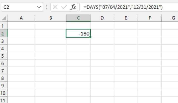 In the example above, the earlier date was entered as the first argument, resulting in a negative integer.
If the date arguments are not considered valid dates, DAYS returns a #VALUE! error.
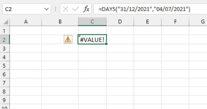 The above date format is considered incorrect for the local date settings, therefore Excel considers these dates invalid and is unable to calculate the difference between the two dates. To correct this, you should either adjust your computer’s regional settings, or change the text input.
6. DAYS360
(Available in Excel 2007 and subsequent versions)
Accounting periods are often based on twelve 30-day months. The DAYS360 function in Excel calculates the number of days between two dates, based on a 360-day year.
Syntax
The syntax of the DAYS360 is:
DAYS360(start_date,end_date,[method])- End_date is one of the two dates being compared.
- Start_date is one of the two dates being compared.
- Method (optional) is a setting, set to TRUE or FALSE, that specifies whether to use the U.S. or European method in the calculation. If omitted, FALSE is assumed.
FALSE is the U.S. (NASD) method. If the starting date is the last day of a month, it’s treated as the 30th day of that month. If the ending date is the last day of a month and the starting date is earlier than the 30th day of a month, the ending date is treated as the 1st day of the next month. Otherwise, the ending date becomes equal to the 30th day of the same month. (Source)
TRUE is the European method. Starting dates and ending dates that occur on the 31st day of a month are treated as the 30th day of the same month.
 In the above example, the ending date (December 31) is treated as the first day of a new month because the starting date (July 4) is earlier than the 30th of the month, so the result is that 177 days have elapsed. When using the European method, the result is 176 days because the ending date is on the 31st day of the month.
7. EDATE
(Available in Excel 2007 and subsequent versions)
The EDATE function returns the date of a future or past month where the day of the month is identical to the date being referenced. The EDATE function may be used to determine maturity, expiry, or due dates. This function returns the serial number of the calculated date, which can then be formatted using the date format of choice.
Syntax
EDATE(start_date,months)- Start_date will be used as the reference date.
- Months is the number of months to be calculated before or after the start_date.
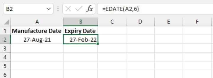 It’s recommended that start_date be entered using the DATE function, or reference the result of a formula or function. Using a text string for the first argument could give unexpected results if Excel does not recognize the values as dates.
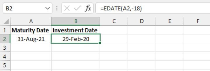
Months can also be entered as a negative value, which will result in subtracting that number of months from the start date, as shown below.
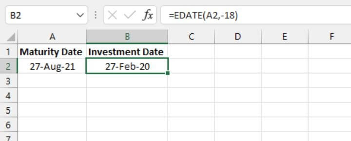
If a number other than an integer is entered in months, EDATE truncates the decimal and uses the whole number value only (see below).
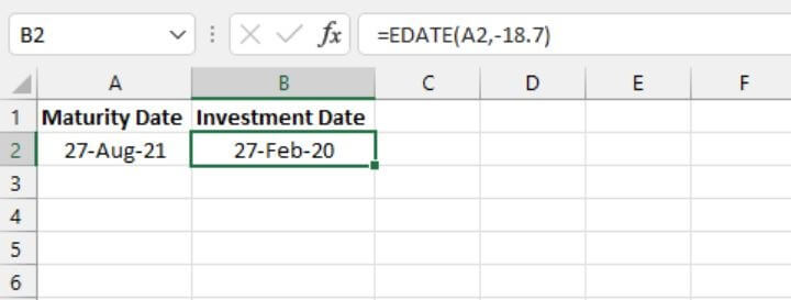 If the resulting month does not have a date with that numeric value, the last day of the month is returned.
8. EOMONTH
(Available in Excel 2007 and subsequent versions)
The EOMONTH function determines the last day of an earlier or later month than the month being referenced. The EOMONTH function may be used to determine maturity, expiry, or due dates when we want to force these to fall on the last day of the month. This function returns the serial number of the calculated date, which can then be formatted using the date format of choice.
Syntax
EOMONTH(start_date,months)- Start_date will be used as the reference date.
- Months is the number of months to be calculated before or after the start_date.
 In the above example, the investment is set to mature on the last date of the month, three years from the investment date.
It’s recommended that start_date be entered using the DATE function, or reference the result of a formula or function. Using a text string for the first argument could give unexpected results if Excel does not recognize the values as dates.
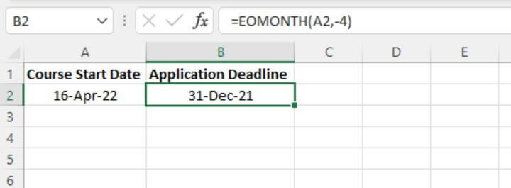
Months can also be entered as a negative value, which will result in subtracting that number of months from the start date, as shown below.
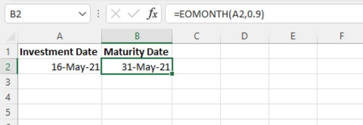
 If a number other than an integer is entered in months, EOMONTH truncates the decimal and uses the whole number value only (see below).
9. ISOWEEKNUM
(Available in Excel 2013 and subsequent versions)
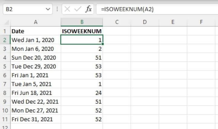
The ISOWEEKNUM function returns the International Organization for Standardization (ISO) week number of the year for the referenced date. The difference between ISOWEEKNUM and WEEKNUM is that ISOWEEKNUM uses the ISO concept of weeks of the year, whereby weeks begin on Monday, and the first week that contains a Thursday is considered Week 1.
Syntax
The syntax of ISOWEEKNUM is:
ISOWEEKNUM(date)The date argument is the serial number that Excel uses to store dates. Date may be a reference to a cell with a serial number formatted as a date, or it may be the result of another Excel function (for example, DATE or TODAY). Using a text string for the date argument could give unexpected results if Excel misinterprets or does not recognize the value as a date.
ISOWEEKNUM returns an integer between 1 and 53.
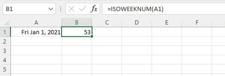 In the above example, the first day of the year is a Friday, so it isn’t considered the first week of the year 2021 but rather, a continuation of the 53rd week of 2020.
 If the date argument isn’t a valid number (for example, a negative number), ISOWEEKNUM returns the #NUM! error value.
If the date argument isn’t a valid date type (for example, 16/16/2021), ISOWEEKNUM returns the #VALUE! error value.
10. MONTH
(Available in Excel 2007 and subsequent versions)
The MONTH function returns the nth month of the year ranging from 1 to 12. This can be useful for isolating the month element of a date.
Syntax
The syntax of the MONTH function is:
MONTH(serial_number)Serial_number is the Excel-assigned number of the date you want to query. The serial number is usually obtained as the result of another Excel function, such as TODAY, DATE, DATEVALUE, etc.
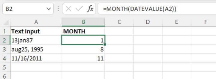 In the image above, the DATEVALUE function was used to identify the dates in column A and convert them into a serial number that Excel would recognize as a date. The MONTH function was then used to extract just the month from each date, and represent that number with a value from 1 to 12.
However, unlike the DAY function, changing the number format in the case of the above output cells isn’t a recommended way to display the name of the month, since Excel does not interpret the output values as a date. A better solution would be to use the TEXT function and use the format_text argument to display the name of each month.
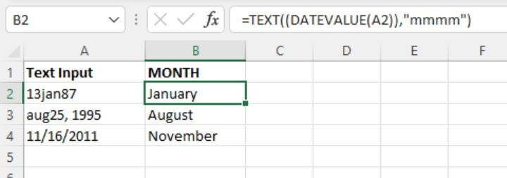 The text format “mmmm” causes the TEXT function to return the full name of the month of the year.
Ready to become a certified Excel ninja?
Start learning for free with GoSkills courses
Explore Excel courses11. NETWORKDAYS
(Available in Excel 2007 and subsequent versions)
NETWORKDAYS is used to determine the number of working days between two dates. The formula calculates the days in an inclusive manner, meaning that the start and end days are included in the count, and Saturdays and Sundays are automatically excluded from the calculation. Additional or ad hoc days may also be excluded using an optional argument.
Syntax
The syntax of the NETWORKDAYS function is:
NETWORKDAYS(start_date, end_date, [holidays])- Start_date is a date that represents the start date.
- End_date is a date that represents the end date.
- Holidays is an optional argument. It can refer to a range of dates to be excluded from the working days calculation. Alternatively, holidays may be explicitly listed within the formula using an array of date serial numbers.
The basic application of NETWORKDAYS is shown below:
=NETWORKDAYS(DATE(2022,1,1),DATE(2022,12,31),B2:B10)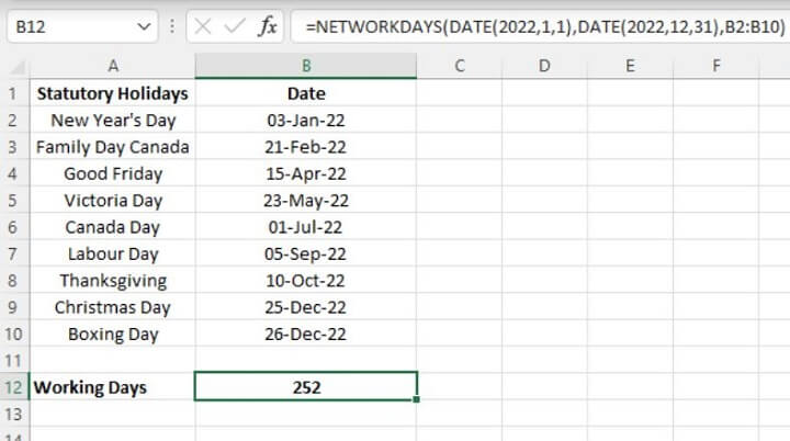 Note that in the above, the DATE function was used for the start_date and end_date arguments. This ensures that Excel does not misinterpret the date, or fail to recognize the values as dates since dates entered as text may lead to incorrect results. For the holidays argument, the range B2:B10 was referenced.
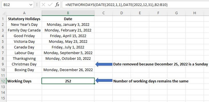
If any date within the holidays argument is a Saturday or Sunday, no additional action is taken by the NETWORKDAYS function; in other words, there is no ‘double-dipping’.
12. NETWORKDAYS.INTL
(Available in Excel 2010 and subsequent versions)
The NETWORKDAYS.INTL function is used to determine the number of whole working days between two dates. The formula calculates the days in an inclusive manner, meaning that the first and last days are included in the count, but weekend days are excluded. Additional or ad hoc days may also be excluded using an optional argument.
This is a concept similar to NETWORKDAYS, but NETWORKDAYS.INTL offers the flexibility of allowing you to control which days of the week are considered weekend days.
Syntax
The syntax of the NETWORKDAYS.INTL function is:
NETWORKDAYS.INTL(start_date, end_date, [weekend],[holidays])- Start_date is a date that represents the start date.
- End_date is a date that represents the end date.
- Weekend is an optional argument. This argument controls the days of the week that are not included in the number of whole working days between start_date and end_date. The weekend argument may be entered as a number string within double quotes or using the Excel-defined number representing when weekends occur. If this argument is omitted, Saturdays and Sundays are assumed to be weekend days.
The basic application of NETWORKDAYS.INTL is shown below:
=NETWORKDAYS.INTL(DATE(2022,1,1),DATE(2022,12,31),,B2:B10)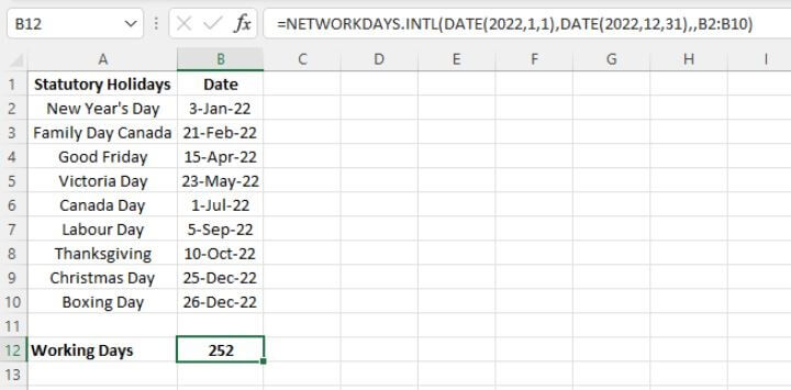 Note that the DATE function was used for the start_date and end_date arguments. This ensures that Excel does not misinterpret the date, or fail to recognize the values as dates. Dates entered as text may lead to incorrect results. For the holidays argument, the range B2:B10 was referenced.
Note also that in the above example, the weekend argument was omitted, and the formula defaulted to Saturdays and Sundays as weekend days. However, if we wanted to designate Fridays and Saturdays as weekend days, we would need to specify this by using the value 7 or the number string “0000110”.
=NETWORKDAYS.INTL(DATE(2022,1,1),DATE(2022,12,31),7,B2:B10)
or
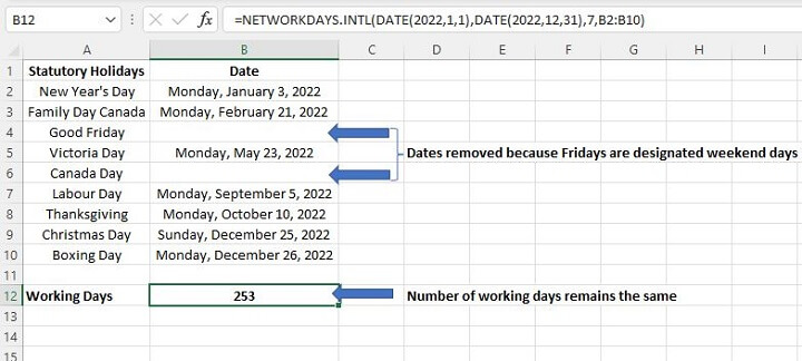
=NETWORKDAYS.INTL(DATE(2022,1,1),DATE(2022,12,31),”0000110”,B2:B10)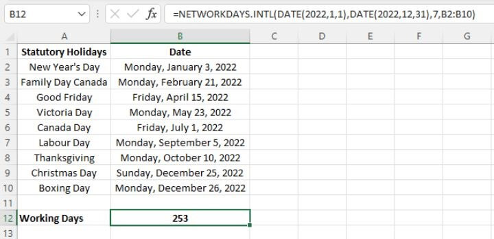 If any date within the holidays argument is a designated weekend day, no additional action is taken by the NETWORKDAYS function. In other words, there is no ‘double-dipping’. See below, where the removal of the April 15 and July 1 dates has no effect since, with Fridays being weekend days, they were already subtracted from the workdays count.
13. NOW
(Available in Excel 2007 and subsequent versions)
The NOW function in Excel returns the serial number of the current date and time. When NOW is used in a cell, a date format matching your computer’s regional settings is applied. The NOW function is considered ‘volatile’, meaning that it updates automatically whenever the worksheet is opened, or when the formulas are manually recalculated.
Syntax
The NOW function has no arguments. The format is:
=NOW()Of course, the number format can be adjusted to display dates and times as per your personal preference by going to the Format Cells dialog box (Ctrl+1 shortcut), then selecting from an available number format from the Date category. Date formats can be further customized by selecting the Custom category.
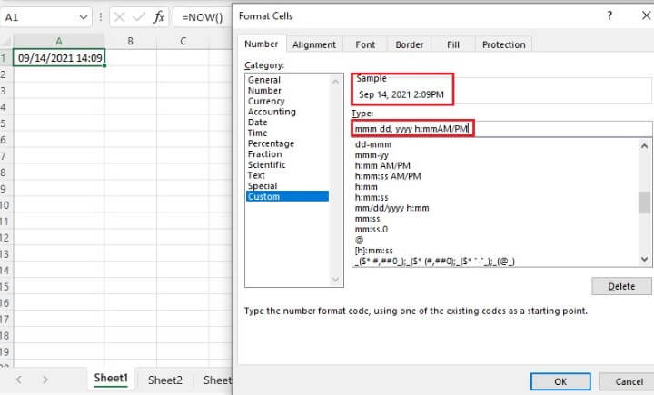 The date and time can be refreshed within an open worksheet by going to the Formulas tab on the ribbon. Then select Calculate Now (F9 shortcut) to recalculate all formulas in the entire workbook. Or select Calculate Sheet (Shift+F9) to recalculate formulas within the current worksheet only.
The NOW function can be modified to create formulas that calculate a future or past date and time relative to the current date and time.
=NOW()+7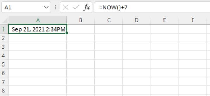 With the above formula, Excel calculates the date and time exactly seven days from now.
If you imagine that the 24 hours making up an entire day is a whole represented by the number 1, then the fraction 0.5 would be equal to half of the day, or 12:00 PM. Various times of the day could also be represented by different fractions (for example 0.25 would be 6:00 AM, 0.95 would be 10:48 PM and so on). Therefore, we can also alter the NOW function to calculate a future or past date and time, which is a fraction of the current date and time.
=NOW()-1.5
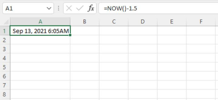 The above formula returns the date and time one and a half days (or 36 hours) prior to the current day and time.
14. TODAY
(Available in Excel 2007 and subsequent versions)
The TODAY function returns the serial number of the current date in Excel. When TODAY is used in a cell, a date format matching your computer’s regional settings is applied. The TODAY function updates automatically whenever the worksheet is opened, or when the formulas are manually recalculated.
Syntax
The TODAY function has no arguments. The format is:
=TODAY()Of course, the number format can be adjusted to display the date as per your personal preference by going to the Format Cells dialog box (Ctrl+1 shortcut), then selecting from an available number format from the Date category. Date formats can be further customized by selecting the Custom category.
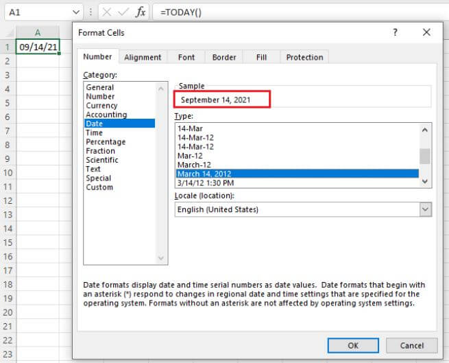 Each time the workbook is opened, the date is recalculated and the current date is displayed. To refresh the date within an open workbook, go to the Formulas tab on the ribbon. Then select Calculate Now (F9 shortcut) to recalculate all formulas in the entire workbook, or select Calculate Sheet (Shift+F9) to recalculate formulas within the current worksheet only. These options are found within the Calculation command group.
The TODAY function can be modified to create formulas that calculate a future or past date relative to the current date.
=TODAY()+7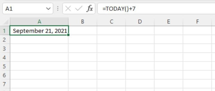 With the above formula, Excel calculates the date seven days from today.
The TODAY function can also be combined with other Excel functions to extract a single element from today’s date, i.e. today’s year, month of the year, or the day of the month.
 With this principle, we can also calculate the number of years elapsed between today and another date.
=YEAR(TODAY())-198315. WEEKDAY
(Available in Excel 2007 and subsequent versions)
The WEEKDAY function returns a number that represents the nth day of the week, ranging from 1 to 7 (or, in some cases, 0 to 6). The function also carries an optional argument that allows you to state the numbers which should represent each day.
Syntax
The syntax of the WEEKDAY function is:
WEEKDAY(serial_number,[return_type])Serial_number is the Excel-assigned number that represents the date you want to query. The serial number is usually obtained as the result of another Excel function, such as TODAY, DATE, DATEVALUE, etc.
Return_type is an optional argument that determines the type of return value. If return_type is omitted, 1 is assumed.
|
Return_Type Argument |
Weekday Values |
|---|---|
|
1 or omitted |
1 through 7, Sunday - Saturday |
|
2 |
1 through 7, Monday - Sunday* |
|
3 |
0 through 6, Monday - Sunday |
|
11 |
1 through 7, Monday - Sunday* |
|
12 |
1 through 7, Tuesday - Monday |
|
13 |
1 through 7, Wednesday - Tuesday |
|
14 |
1 through 7, Thursday - Wednesday |
|
15 |
1 through 7, Friday - Thursday |
|
16 |
1 through 7, Saturday - Friday |
|
17 |
1 through 7, Sunday - Saturday |
*The WEEKDAY function is available in all Excel versions, but only return_types 1, 2, and 3 were available before Excel 2010. Return_types 2 and 11 are identical in functionality.
Basic application
This function can be used to identify the day of the week on which a particular date falls. Each day of the week is represented by a number, the default being that the number 1 represents Sunday, 2 represents Monday, and so on.
=WEEKDAY(DATE(1979,8,14)) The above formula asks Excel to check the date August 14, 1979 and return the number which represents the day of the week. Since no return_type was entered, Sunday is considered the first day of the week and is represented by the number 1. Therefore, the return value of 3 means that date was a Tuesday.
The serial number may also refer to a date value in another cell. In the example below, the date is entered in cell A1. Excel recognizes this entry as a date value, converts the value to the date’s serial number, and displays the date in a format accepted by the computer’s regional date settings.
 In the background, Excel has stored the date as a unique serial number representing the date that is the result of the calculation. If you change the number format to General, the serial number will be displayed.
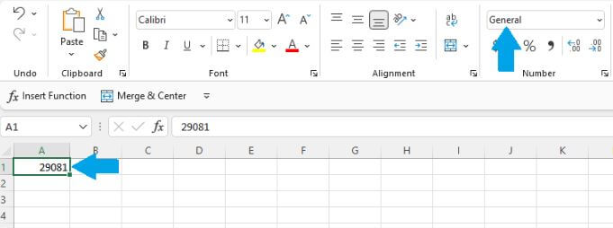 From this, you can see that we can now reference cell A1 with the WEEKDAY function to determine what day of the week that date was.

Display day of the week by name
The value returned by the WEEKDAY function can be converted to display the weekday name by adding the TEXT function.
=TEXT(WEEKDAY(A1),”ddd”) Using the 4-character code “dddd” will result in the full name of the weekday. This method works well when Sunday is the designated first day of the week.
When Sunday isn’t the first day of the week
In some settings, a day other than Sunday is considered the first day of the week. For example, in some workplaces, Monday is designated as the first day of the week, and Sunday as the last. In those cases, it may be preferable to use the return_type argument of the WEEKDAY function to identify the weekday on which a particular date falls.
=WEEKDAY(DATE(2022,1,1),2)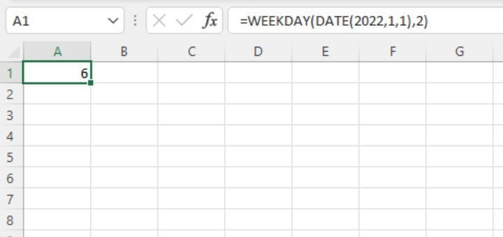 Since 2 was used as the return_type of the WEEKDAY function, an output of 6 means that January 1, 2022 is a Saturday. It’s very important to point out that when the week begins on a day other than Sunday, the TEXT function will not return the correct value for the name of the weekday.
One workable solution is to use the SWITCH function to declare alternate values for each possible result.
The syntax of the SWITCH function is:
=SWITCH(expression, value1, result1, [default or value2, result2],…[default or value3, result3])In this case, we will not use a default value, since the result of the WEEKDAY formula will always fall between 1 and 7.
=SWITCH(WEEKDAY(A2,2),1,"Monday",2,"Tuesday",3,"Wednesday",4,"Thursday",5,"Friday",6,"Saturday",7,"Sunday")16. WEEKNUM
(Available in Excel 2007 and subsequent versions)
The WEEKNUM function returns the week number of the year for the referenced date. The difference between ISOWEEKNUM and WEEKNUM is that WEEKNUM uses two possible systems to determine the week number, whereas ISOWEEKNUM uses the ISO standard.
- With System 1, the week containing January 1 is always considered Week 1.
- With System 2, the week containing the first Thursday of the year is considered Week 1. This system is commonly known as the European week numbering system and is the one used with the ISOWEEKNUM function.
WEEKNUM returns an integer between 1 and 54.
Syntax
The syntax of WEEKNUM is:
WEEKNUM(serial_number, [return_type]))
- Serial_number is a unique number that Excel uses to store each date.
- Return_type is an optional argument that determines the type of return value. If return_type is omitted, 1 is assumed.
The following options are available options for the return_type argument.
|
Return_type Argument |
Week Begins on |
System |
|---|---|---|
|
1 or omitted |
Sunday |
1 |
|
2 |
Monday* |
1 |
|
11 |
Monday* |
1 |
|
12 |
Tuesday |
1 |
|
13 |
Wednesday |
1 |
|
14 |
Thursday |
1 |
|
15 |
Friday |
1 |
|
16 |
Saturday |
1 |
|
17 |
Sunday |
1 |
|
21 |
Monday |
2 |
*The WEEKNUM function is available in all Excel versions, but only return types 1 and 2 were available before Excel 2010. Return types 2 and 11 are identical in functionality.
Basic application
In its default setting, WEEKNUM assumes that the week begins on a Sunday. If the first day of the year is a Sunday, January 1-7 are considered Week 1. If the first day of the year is any day other than a Sunday, Week 1 would begin on January 1 and end on the first Saturday of the year. Week 2 would begin on the first Sunday of the year.
=WEEKNUM(A2)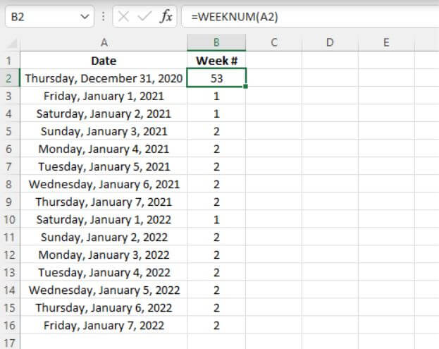 If Monday is the designated first day of the week, return_type 2 should be selected.
=WEEKNUM(A2,2)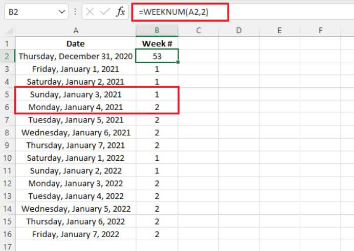 Return_type 21 behaves very differently, whereby Week 1 will be the first week containing a Thursday. Otherwise, the week number will continue from the previous year, and the week begins on Monday. With this setting, WEEKNUM behaves the same as the ISOWEEKNUM function.
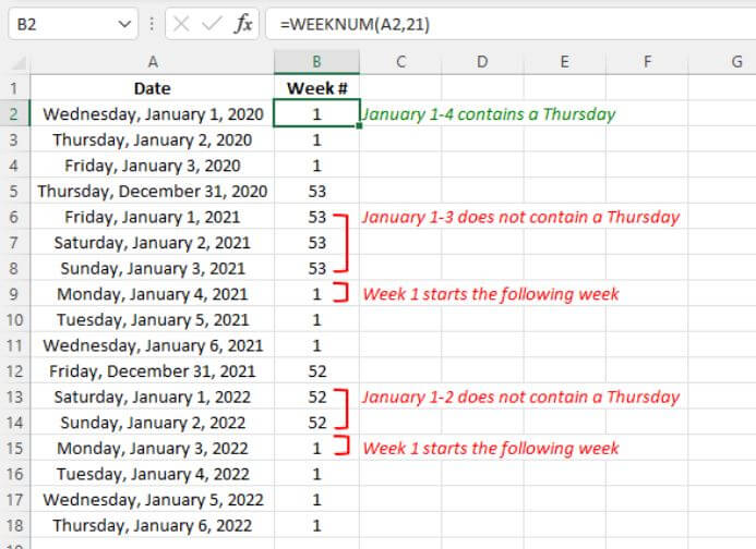 If the date argument isn’t a valid number (for example, a negative number), WEEKNUM returns the #NUM! error value.
If the date argument isn’t a valid date type (for example, 16/16/2021), WEEKNUM returns the #VALUE! error value.
17. WORKDAY
(Available in Excel 2007 and subsequent versions)
The WORKDAY function calculates the date, which is n number of working days before or after a starting date. The starting date isn’t included in the number of days being counted. Saturdays and Sundays are automatically excluded from the count. Holidays may also be excluded using an optional holiday argument.
Syntax
WORKDAY(start_date, days, [holidays])
- Start_date is the date to be used for reference.
- Days is the number of days to add to or subtract from start_date. Saturdays and Sundays are ignored if they fall within the range of days. A negative days value will result in a past date.
- Holidays is an optional argument. It can refer to a range of one or more dates to be excluded from the working days calculation. Alternatively, holidays may be explicitly listed within the formula using an array of date serial numbers.
Basic application
WORKDAY is typically used to calculate the end date of a project when the estimated number of workdays is known. An example is shown below.
 Since the project spans a Saturday and a Sunday, these days are not included in the seven-day count and the project will end nine calendar days after the start date.
The use of the optional holiday argument allows additional days to be excluded from the number of working days.
=WORKDAY(D2,E2,B2:B10)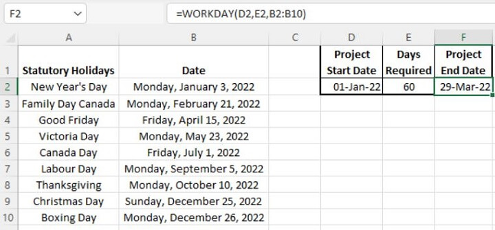
18. WORKDAY.INTL
(Available in Excel 2010 and subsequent versions)
The WORKDAY.INTL function returns the serial number of the date, which is the specified number of working days before or after a starting date. This function is similar to the WORKDAY function, but WORKDAY.INTL offers the flexibility of allowing you to control which days of the week are considered weekend days.
Syntax
The syntax of the WORKDAY.INTL is:
WORKDAY.INTL(start_date, days, [weekend], [holidays])
- Start_date is the start date to be used as a reference.
- Days is the number of days to add to or subtract from start_date. Saturdays and Sundays are ignored if they fall within the range of days. A negative days value will result in a past date.
- Weekend is an optional argument. This argument controls the days of the week that aren't included in the number of whole working days between start_date and end_date. The weekend argument may be entered as a number string, or by using the Excel-defined number representing when weekends occur. If this argument is omitted, Saturdays and Sundays are assumed to be weekend days. See the table below for possible values for the weekend argument.
- Holidays is also an optional argument. It can refer to a range of one or more dates to be excluded from the working days calculation. Alternatively, holidays may be explicitly listed within the formula using an array of date serial numbers.
|
Weekend Argument Value |
Weekend Day(s) |
|---|---|
|
1 or omitted |
Saturday, Sunday |
|
2 |
Sunday, Monday |
|
3 |
Monday, Tuesday |
|
4 |
Tuesday, Wednesday |
|
5 |
Wednesday, Thursday |
|
6 |
Thursday, Friday |
|
7 |
Friday, Saturday |
|
11 |
Sunday only |
|
12 |
Monday only |
|
13 |
Tuesday only |
|
14 |
Wednesday only |
|
15 |
Thursday only |
|
16 |
Friday only |
|
17 |
Saturday only |
Alternatively, the weekend argument may be represented by a number string entered within double quotation marks where weekend days are represented by the number 1, and workdays are represented by 0. Monday is the first day of the week in the number string. Using this system, the number string “0000110” represents a week where Friday and Saturday are weekend days.
Basic application
WORKDAY.INTL is typically used to calculate the end date of a project when the estimated number of workdays is known, especially when weekend days aren’t the default Saturday and Sunday combination. An example is shown below, where Sundays are to be considered weekend days.
=WORKDAY.INTL(A2,B2,11) The weekend argument is given a value of 11 since Sundays are the only days to be considered weekend days. Since the project spans a Sunday, that day isn’t included in the seven-day count and the project will end eight calendar days after the start date.
The use of the optional holiday argument allows additional days to be excluded from the number of working days.
=WORKDAY.INTL(D2,E2,11,B2:B10)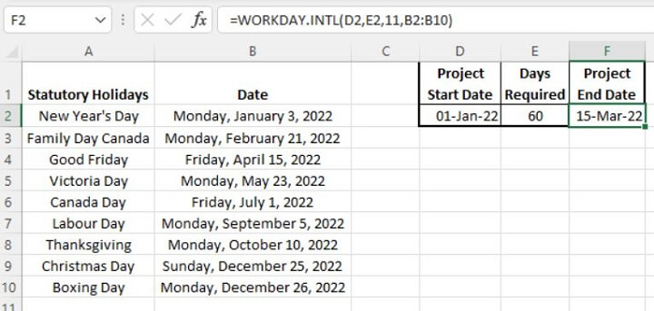
When no days should be excluded
What if you would like to calculate the end date without excluding any weekend days or holidays? Perhaps the project will be worked on every day until completion. In that case, the DAYS function should be used instead.
19. YEAR
(Available in Excel 2007 and subsequent versions)
The YEAR function returns the year corresponding to a date. This can be useful for isolating the year element of a date.
Syntax
The syntax of the YEAR function is:
YEAR(serial_number)Serial_number is the Excel-assigned number of the date you want to query. The serial number is usually obtained as the result of another Excel function, such as TODAY, DATE, DATEVALUE, etc.
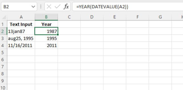 In the image above, the DATEVALUE function is used to identify the dates in column A and convert them into a serial number that Excel would recognize as a date. The YEAR function is then used to extract just the year from each date.
Get your FREE cheatsheet!
Download your printable cheatsheet with 20 Excel date functions here.
20. YEARFRAC
(Available in Excel 2007 and subsequent versions)
The YEARFRAC function calculates the number of days between two dates (the start_date and the end_date) as a fraction of the entire year. The output value is a decimal. This function can be useful for calculating one’s age to a fraction.
Syntax
The syntax of the YEARFRAC function is:
YEARFRAC(start_date, end_date, [basis])
- Start_date is one of the two dates being compared.
- End_date is one of the two dates being compared.
- Basis is an optional argument that controls the type of day count to be used. See the table below for possible options.
|
YEARFRAC Basis Value |
Calculation |
Remarks |
|---|---|---|
|
0 or omitted |
30/360 |
US system |
|
1 |
# of days/days in the year |
|
|
2 |
# of days/360 |
|
|
3 |
# of days/365 |
|
|
4 |
30/360 |
European system |
Both the U.S. and European systems assume years consisting of twelve 30-day months.
The U.S. (NASD) method assumes a year to consist of twelve 30-day months. If the starting date is the last day of a month, it’s treated as the 30th day of that month. If the ending date is the last day of a month and the starting date is earlier than the 30th day of a month, the ending date is treated as the 1st day of the next month. Otherwise, the ending date becomes equal to the 30th day of the same month (Source).
The European method also assumes a year to consist of twelve 30-day months. However, starting dates and ending dates that occur on the 31st day of a month are treated as the 30th day of the same month.
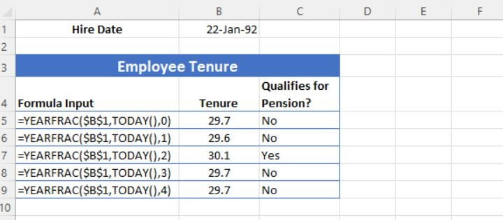
Conclusion
Now you understand how Excel dates work and how you can simplify the way they are processed with one of these incredibly useful Excel DATE functions.
To learn more Excel, try our courses, including one of our most popular courses Microsoft Excel - Basic to Advanced.
Ready to become a certified Excel ninja?
Start learning for free with GoSkills courses
Explore Excel courses
