The Excel Ribbon

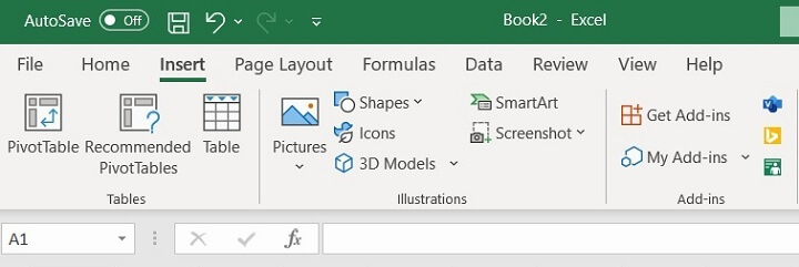
What is the Excel ribbon?

The Excel ribbon refers to the tabs at the top of the Excel interface that helps users to navigate and locate the commands when using Excel.

---

Learn Excel for free

Start learning formulas, functions, and time-saving hacks today with this free course!

Start free course

---

The Excel ribbon tabs

There are nine tabs on the Excel Ribbon: File, Home, Insert, Page Layout, Formulas, Data, Review, View, and Help. The Home tab is the default tab when Excel is opened.

Now let’s go through each tab, from left to right, to understand each of their features.

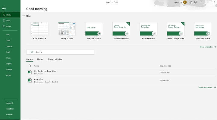
1. File

This provides a backstage view of all the important commands related to the files — to create a new sheet, open a file, save the file, print the file, and export.

2. Home

This features the essential or most frequently used commands in Excel — formatting, font types, and filtering. 

Similar features are organized by group, for example there is a Clipboard group with cut, copy, and paste commands; and a Font group with font styles, colors, and sizes.

Note that your ribbon options may appear differently depending on how big your screen is, and the size of your Excel window (as you make it smaller, you'll notice less buttons appear).

As there are a lot of features, we have divided it into two sections as pictured below, to give you a better look at all the buttons and groups.

3. Insert

This is where users can add various items to a spreadsheet, including Pivot Tables, pictures, shapes, charts, graphs, and symbols.

4. Page Layout

This allows users to customize the layout of the spreadsheet by adjusting the margins, color themes, gridlines, and print area. The changes are applicable when being printed as well.

5. Formulas

This is where all essential formulas are categorized under the function library and it provides various controlling options.

6. Data

This allows users to manage data in the current spreadsheet, within the file, and also to import external data from other sources.

7. Review

This is for users to perform various controlling functions, including spell check, translate, adding comments and notes, track changes, and to enable worksheet protection.

8. View

This provides options to alter the views of worksheets — gridlines, zoom, freeze panes, and to switch windows.

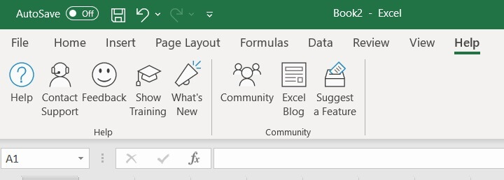
9. Help

This gives access to Microsoft support. It allows you to provide feedback and to suggest a feature to the community.

How to collapse and to restore the ribbon in Excel

By default, the ribbon is a “fixed” feature in Excel, meaning that it stays in the same place as we scroll down the page. However, when working on a large set of data in Excel, we might want to get extra space on the screen.

To do that, we can collapse the ribbon without having to zoom out or change the font size of the data or text.

How to collapse the ribbon in Excel

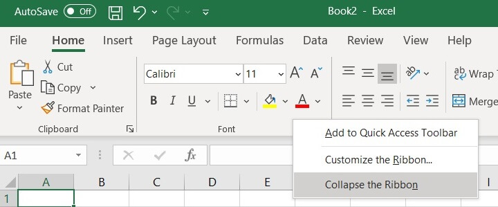
To collapse the ribbon in Excel: 

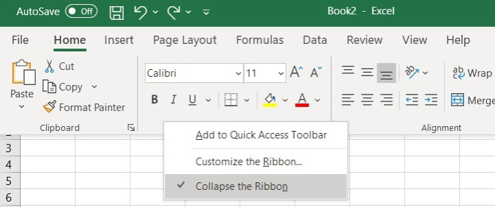
1. Right click anywhere on the ribbon. 
2. Then select the last option — Collapse the Ribbon.

The ribbon has been hidden.

If you click on any of the commands (File, Home, Insert, Page Layout, etc.,) the relevant Excel ribbon will appear.

How to restore the ribbon in Excel

You can restore the ribbon in exactly the same way we collapse the ribbon.

1. Click on any command to access the ribbon. 
2. Right click anywhere and unselect Collapse the Ribbon.

---

---

How to customize the ribbon in Excel

As the Excel ribbon features most of the most frequently used commands, a customized ribbon helps ensure a smoother and faster user experience in Excel.  

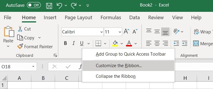
To customize the ribbon in Excel, just like collapsing the ribbon, right click anywhere on the ribbon and select Customize the Ribbon instead.

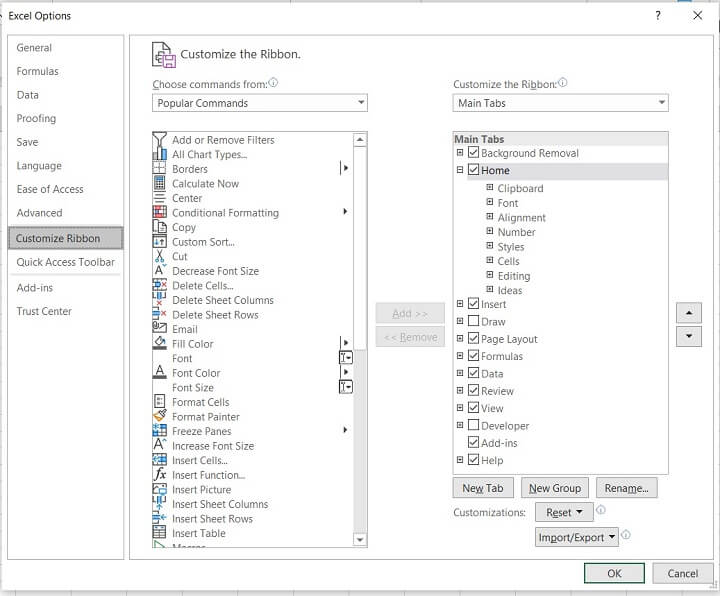
The window below will pop up and it allows users to customize the ribbon by adding or removing the commands to or from the existing tabs or new tabs.

To add a command to a new tab

1. Click New Tab. A new tab will be created under the Main Tabs section.

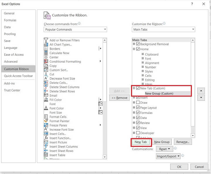
2. Rename it if you wish by clicking Rename and then input the name. We’ve used “Goskills” in this example:

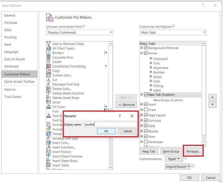
3. Click OK.

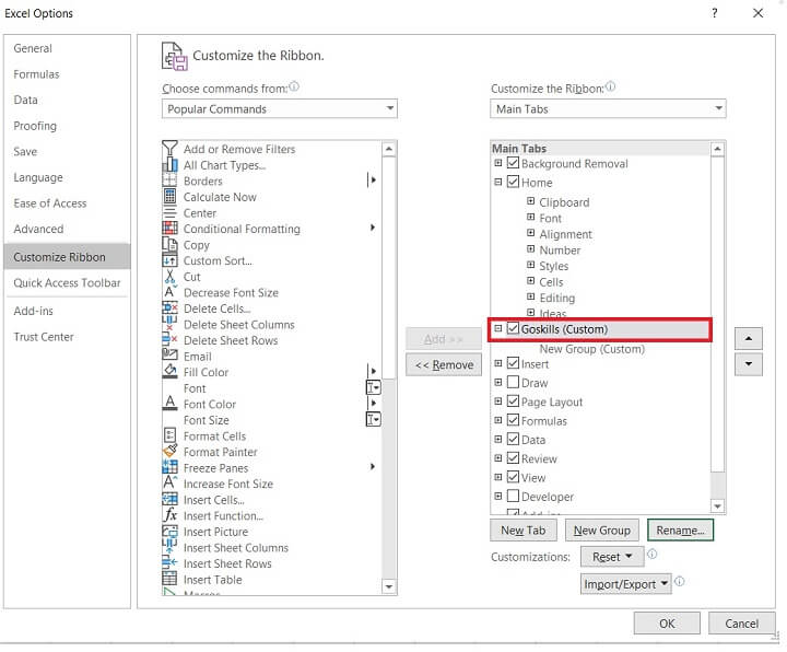
4. Select any command (e.g. Insert Picture) and add under the Group.

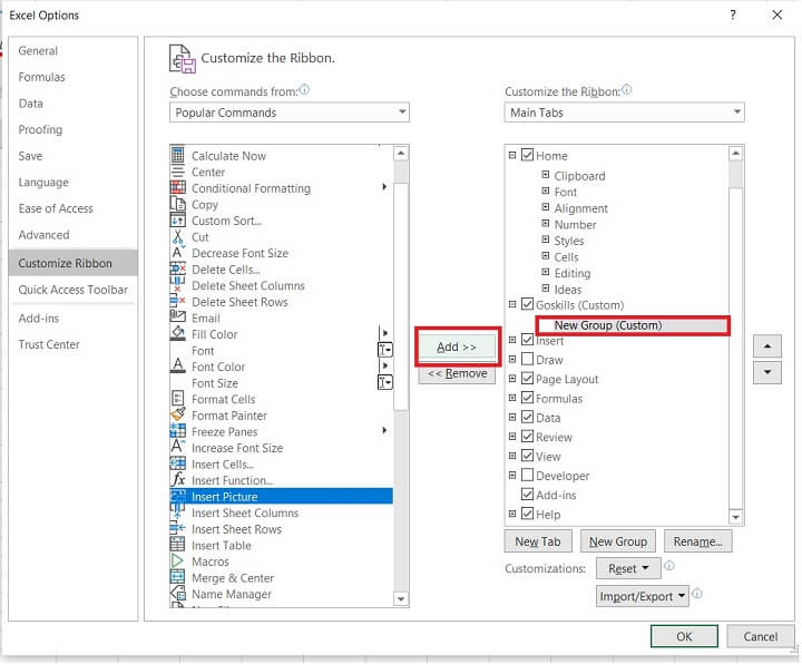The command (Insert Picture) is now under a group under the new tab (Goskills).

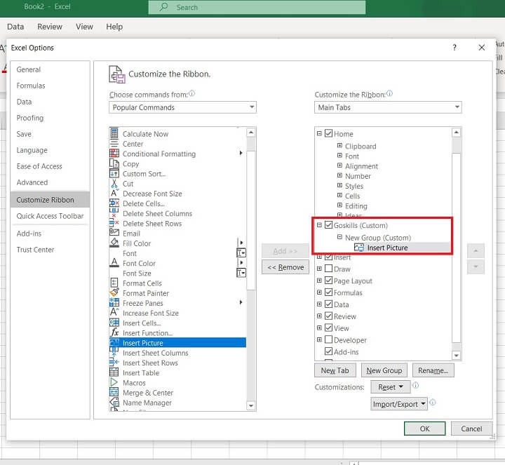
5. Click OK at the bottom right to confirm the customization.

A new tab named GoSkills is now the one to the right of the Home tab. Under the tab, there’s a group with one command — Insert Picture.

Note: Users can customize the name of the group as well. The steps are the same as renaming the name of the tab.

To reset the Excel Ribbons

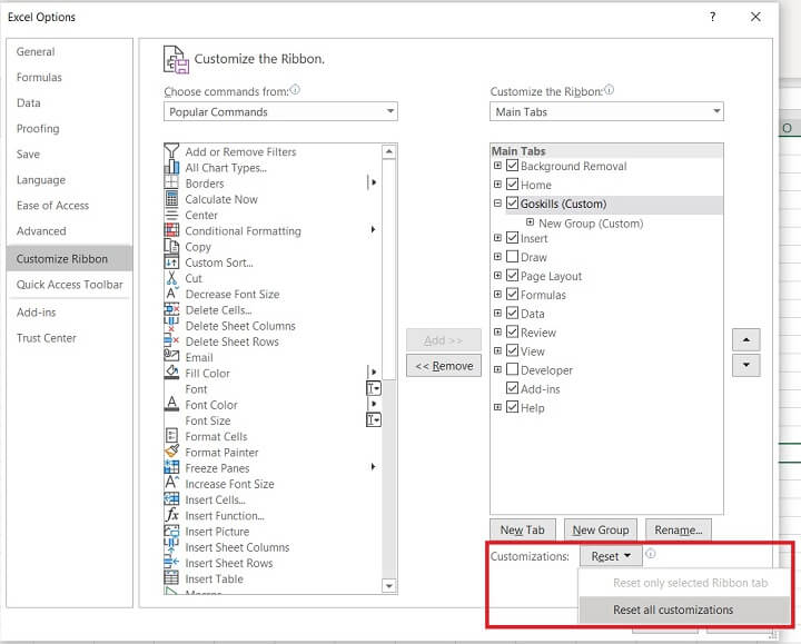
It’s equally important to reset and undo the customization as it is to customize. To reset:

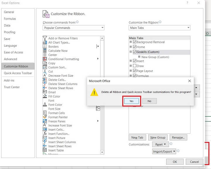
1. In Excel Options, select Reset All Customizations under Customizations.

2. Click Yes and then OK at the right bottom.

Auto-hide ribbon and show tabs and commands

At the top left corner of the Excel window, there are shortcuts available for the display of the Excel ribbons.

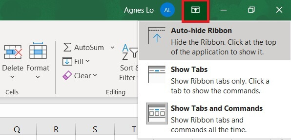
• Select Auto-hide Ribbon to hide both tabs and commands.

• Select Show Tabs to show Ribbon tabs only.

• Select Show Tabs and Commands for the default view of both Ribbon tabs and commands readily available on display.

Ready to learn more Excel essentials?

Excel Ribbon tabs and commands are the most frequently used features in Excel. 

They cover features from formatting, to layouts, creating graphs, and sorting and analyzing data. You can customize your ribbon to facilitate your work in Excel. 

To learn more Excel essentials, try our free Excel in an Hour course today!

This beginner friendly course will teach you the basics of Excel and how to master essential functions and formulas in just one hour. ⌚

Learn Excel for free

Start learning formulas, functions, and time-saving hacks today with this free course!

Start free course