Microsoft Excel is one of the world's most popular business software packages. It is incredibly powerful, and its features regularly get an upgrade to make it even better.
You might be trying to learn how to master Excel – regardless of your job role, Excel can help you work quicker, smarter, and with more efficiency. This article will guide you through 12 of the best tips and tricks to help you harness the power of Excel and impress your boss and work colleagues.
How to master Excel fast in 12 steps
1. Get comfortable navigating the interface
Need a place to start? Here's our recommendation: Learn how to navigate the Excel interface.
Let’s start with the basics:
When typing data into Excel you can use the Tab key to move to the next cell in the column to the right.
You can use Enter to move to the cell in the next row down. If you have been using tab to move through the columns, pressing Enter will take you one row down and back to the cell in the column you started in.
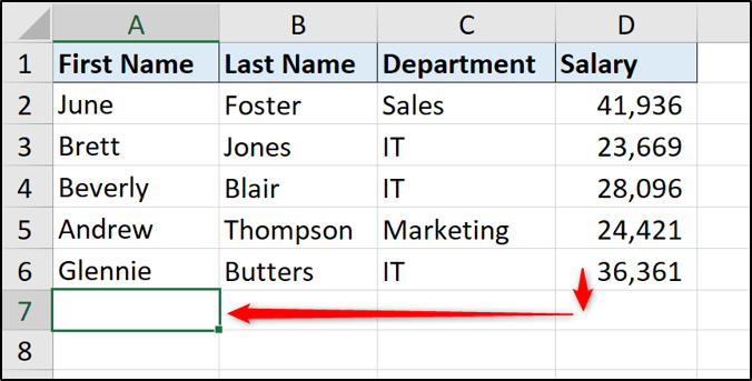
Pressing the Ctrl key and the Up, Down, Left or Right directional arrow keys together will take you to the last used cell in that direction. This is very useful to navigate large lists on Excel.
Pressing the Ctrl and the Home key together will take you to the first cell in your data range.
2. Learn some useful shortcuts
The best way to speed up your day-to-day Excel work is to learn some useful shortcuts both with the keyboard and your mouse or touchpad.
If you're a beginner, then start by learning the general keyboard shortcuts. Some good ones to learn are the famous copy and paste: Ctrl + C to copy and Ctrl + V to paste. Plus, there's Ctrl + Z to undo the last action – great for any accidental actions!
As you begin to use these Excel shortcuts in your daily work, push yourself to learn more.
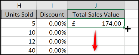
Two of my favorite shortcuts are Ctrl + ; to enter today's date in a cell. And double-clicking the fill handle (the square in the bottom right corner of the cell) to copy to the bottom of a list.
Excel has over 500 keyboard shortcuts and a whole bunch of useful tricks for speeding up how you work.
Although you won’t need them all, learning some to make your Excel work easier is a great idea.
Ready to start using Excel shortcuts?
Download our printable shortcut cheatsheet for Excel.
3. Freeze panes
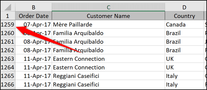
Freezing panes is a handy Excel feature that keeps your headings and other labels visible at all times as you scroll around the spreadsheet. It's an essential skill to know.
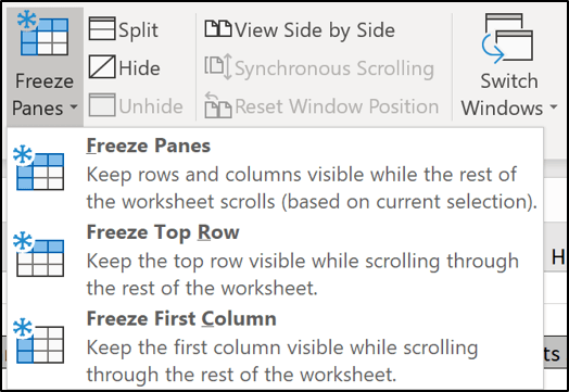
The headings for a spreadsheet are usually just in the top row. So to freeze this area, click View > Freeze Panes > Freeze Top Row.
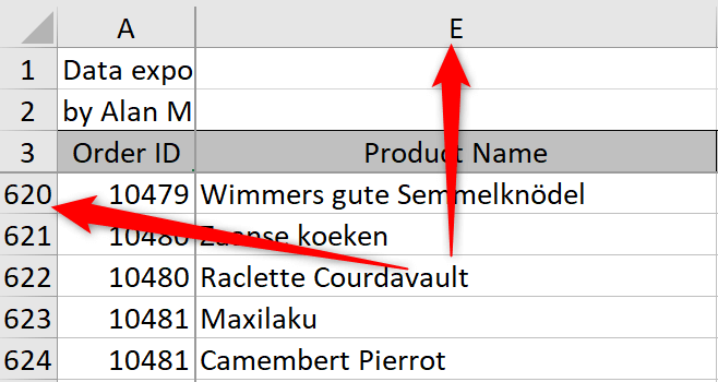
In the image below, we are looking at row 1259 but the headings are still visible on screen.
You can freeze as many rows, and columns, as you need.
Click in the first cell after the rows and columns you want to freeze. For example, if you want to freeze 3 rows and 1 column, click on cell B4.
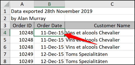
Click View > Freeze Panes > the first Freeze Panes option.
Now when you scroll down, the first 3 rows remain visible. And if you scroll to the right, column A remains visible.
4. Understand Excel formulas
One of the main ways to master Excel is to be accomplished at writing formulas. These are the muscles of Excel.
Whether it's performing basic calculations in cells or using more advanced formulas, if you know how to use these functions, you will stand head and shoulders above the rest!
If you aren't sure where to begin, start with creating basic calculations that add, subtract, multiply, and divide values. Then begin to learn some of the more commonly used functions. These include SUM, IF, VLOOKUP, COUNTIF, and CONCATENATE.
Once you are comfortable writing formulas, you can do almost anything. You can even use formulas within Conditional Formatting rules, charts, and other Excel features to make them more powerful.
Check out some of our favorite Excel formulas and functions.
5. Learn how to create a simple drop-down list
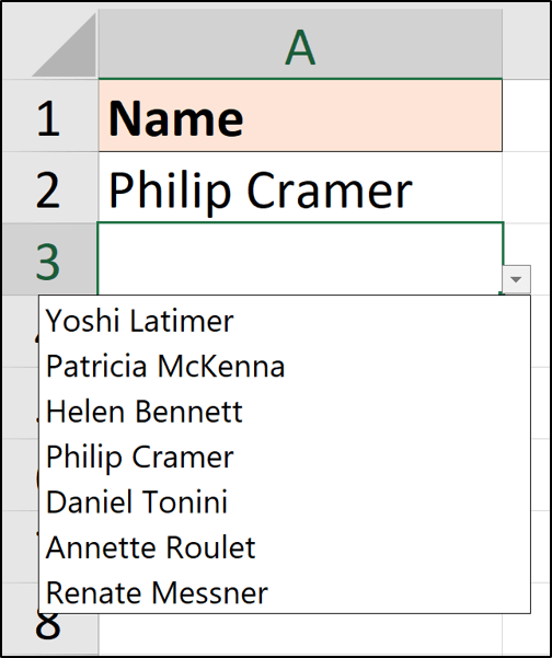
A simple Excel dropdown list on a spreadsheet can make entering text much easier and, more importantly, ensure it is accurate.
To create an Excel dropdown list;
1. Select the range of cells you want the list to appear in.
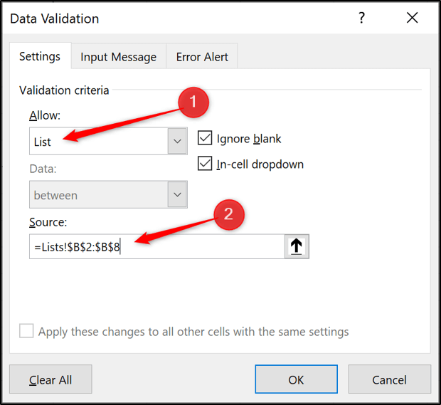
2. Click Data > Data Validation.
3. Select List from the Allow list.
4. Then either type the list items into the source box separating each one with a comma. Or select a range of cells that contain the list items.
Now you have a drop-down list, making data entry simple and reliable.
6. Visualize key data with conditional formatting
Conditional Formatting is one of the most popular features of Excel. It helps the user get a quick understanding of the data they are looking at.
You can create simple conditions to automatically format cells if a target is reached, a deadline has passed or maybe sales have decreased below a certain threshold.
For a quick example, if a value is larger than 300 we want to change the cell color to green.
1. Select the range of cells that you want to apply Conditional Formatting to.
2. Click Home > Conditional Formatting > Highlight Cells Rules > Greater Than.
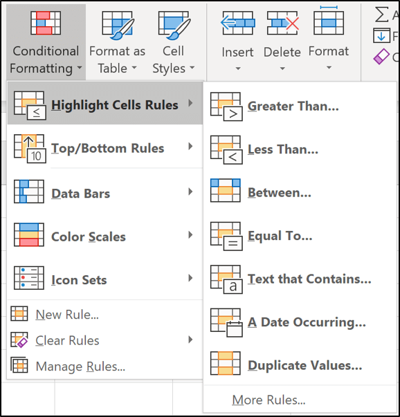
3. Enter 300 and select the formatting you want to apply.
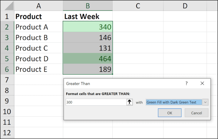
A green fill and font color are used here, but there are lots of formatting options available.
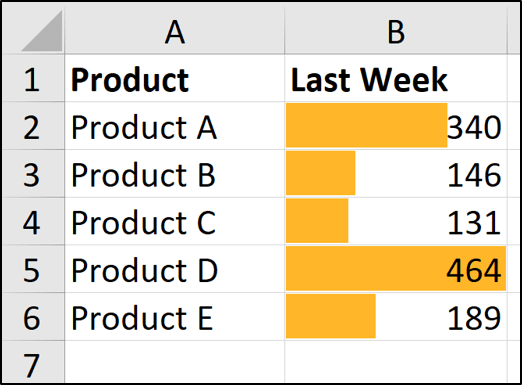
With conditional formatting on Excel, there is also the ability to apply data bars and icon sets. These visuals can be very effective. The image below shows data bars applied to the same range of values.
7. Get things done faster with Flash Fill
Flash Fill is an awesome Excel feature that quickly manipulates data. This feature can greatly reduce the time taken doing regular data cleansing tasks, which previously we relied on Excel formulas and macros to do.
Take, for example, the list below. We want to extract the name from the list in column A.
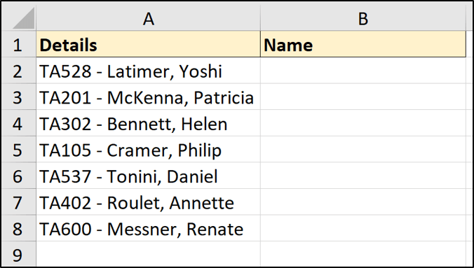
Enter the first name in cell B2 and then the second name in cell B3 and as you type, Flash Fill picks up the pattern in your behavior asks if you would like it repeated over the rest of the rows. This is amazing!
Press Enter and voilà the data is extracted.
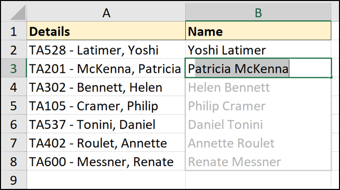
There are several ways of running Excel Flash Fill. You can also find the button on the Data tab of the Ribbon, and you can operate it with the shortcut Ctrl + E.
8. Learn visual storytelling with charts and graphs
Learning how to represent numerical data with pictures is definitely a skill you should master if you want to be proficient in Excel. Not everyone will want to inspect and compare endless rows of data for patterns and trends. Mastering Excel data visualization will make it easy for you to highlight the most important bits of information in your dataset.
Here’s how to create a graph in Excel in 3 easy steps:
1. Highlight the source data.
2. Go to Insert on the Excel ribbon and select the type of graph you want.

3. Use the available customization options to format the chart the way you want.
Chart customization
The ways in which you can customize a chart in Excel are virtually endless. The Chart Design tab is contextual, meaning it only appears when a chart is selected. Using this menu option, you can change the style, source, or location of your chart, and you can also add additional elements like a legend, data labels, and axis titles.


🚀Need to learn the basics of Excel fast? This free, 1-hour Excel crash course is exactly what you need.
9. Summarize data with PivotTables
Pivot tables are some of the most amazing tools in Excel. They make summarising large datasets as easy as 1, 2, 3.
An Excel PivotTable could be used to break down an extensive list of sales to see the sales by region or even sales of particular products in each region.
They're extremely powerful, but also simple to use. A PivotTable is an Excel tool to make creating reports more straightforward and doesn't require writing any complex formulae.
To create a PivotTable:
1. Click on the list of data you want to summarize.
2. Click Insert > PivotTable.
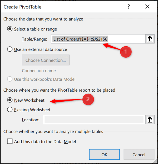
3. In the Create PivotTable dialog, ensure the range being used is correct and specify whether you want the PivotTable or a new or existing worksheet.
4. Drag and Drop fields from the field list into the four areas to create your Excel PivotTable.
In the image below, the years is in Columns, the product category in Rows and the total sales value in the Values area.
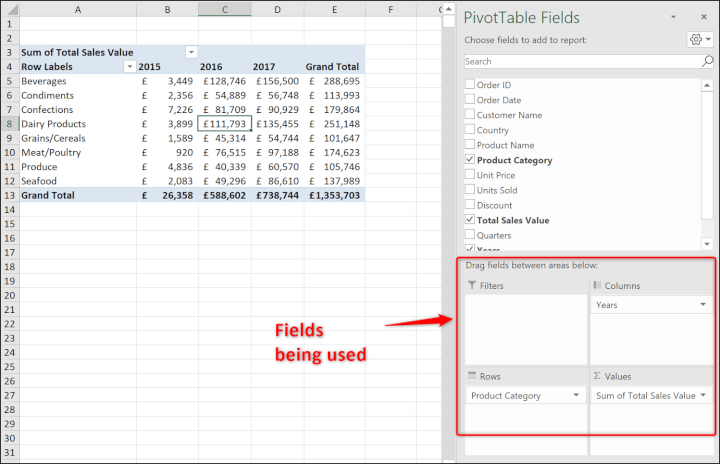
The Excel Values area is where the calculations such as sum, count and average are performed.
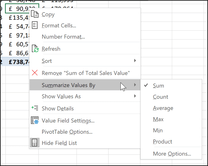
The calculation can be changed by right-clicking a PivotTable value, selecting Summarize Values By and selecting the Excel function you want to use.
There is plenty more that Excel PivotTables offer but that is beyond the scope of this article.
With PivotTables, I encourage you to grab some spreadsheet data, insert a PivotTable and start to drag fields into the areas and explore the options available. Excel is really is a tool that you learn by doing.
10. Learn how to protect worksheet data
Excel features such as PivotTables, formulas, and conditional formatting will only work if the data is accurate.
A few of the tips in this article demonstrate ways to maintain this accuracy, including creating drop-down lists and using Flash Fill. Protecting your data is another important step to take.
Excel has a few different types of protection that can be applied, but the most popular one is to protect the sheet.
Protecting a sheet is performed in two stages. Firstly you specify which cells on the worksheet, you do not want to lock. This ensures that users can still edit these cells. Then you apply the protection.
- Select the range(s) of cells that you want to unlock (hold down the Ctrl key to select multiple ranges at the same time).
- Press Ctrl + 1 to open the Format Cells dialog.
- Click the Protection tab, uncheck the Locked box and click Ok.
- Click Review > Protect Sheet.
- You can enter a password for extra security, but it is optional (this is typically omitted as you are normally protecting against accidents and a password is unnecessary). Check the boxes of any functionality users will need to perform and click Ok.
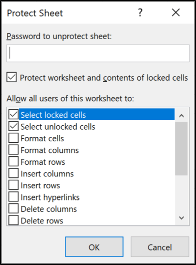
The unlocked cells can still be changed, but with limited functionality. If you try and edit a locked cell, a message will appear telling you that the sheet is protected.

11. Power up with Power Query and Power Pivot
Having knowledge of these two Power tools will take you beyond the regular user.
Power Query is a tool used to import and shape data ready for analysis. It is found on the Data tab of the Ribbon.
With Power Query, you can import data easily from a variety (and constantly evolving) of places including CSV, the web and from a folder.
The Power Query Editor then provides a user-friendly environment to perform a number of cleaning and shaping operations such as splitting columns, formatting, removing duplicates and unpivoting data.
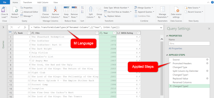
Power Query uses a language called M. This is difficult to master and fortunately not needed for 99% of Excel users. The editor provides everything that a user would need.
Every edit that is made is stored as a step and can be refreshed in the future with the click of a button.
Power Pivot (also known as the data model) is a tool that enables the storage of huge volumes of data. Storing data in Power Pivot enables us to go beyond the physical limitations of Excel.
In Power Pivot you can also create relationships between multiple tables of data and write functions known as DAX function.
The ability to create these models and use DAX provides far more power than you can get more a spreadsheet.
This is an important tool to understand for anyone involved in analyzing huge quantities of data or needs to perform complex analysis.
Bonus: Check out Ken Puls' lesson from his Power Pivot course which explains what Power Pivot is, and how it can streamline your workflow.
12. Create Macros with VBA
Macros in Excel enable you to automate repetitive tasks to supercharge your productivity.
These tasks can be complex, but for most users, they are reasonably simple tasks that are repeated often. Macros provide a way to perform tasks quicker and more reliably.
You can get started with macros by recording yourself performing Excel tasks. This will generate the VBA code and produce a macro.
You can find the macro recorder on the View tab of the Ribbon. It is the last button.
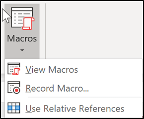
Recording Excel macros can save you and your colleagues a great deal of time.
If you want to take things further, you can learn Excel VBA and edit your macros.
With VBA you can make your macros do things way beyond recording and create functionality that Excel does not offer itself.
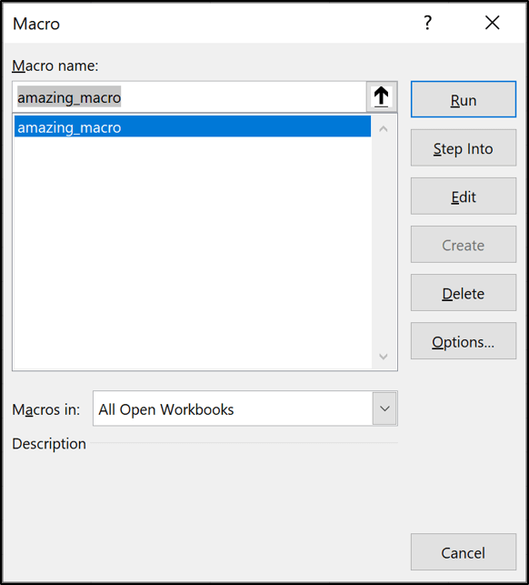
To see the VBA code created by a recording;
Click View > Macros, select the macro in the list and click Edit.
Want to master Excel?
Of all the tips on how to master Excel, the best way is to take a structured online Excel course that teaches you everything you need to know. Practice alongside a Microsoft MVP and learn the latest skills to boost your workplace efficiency!
Level up your Excel skills
Become a certified Excel ninja with GoSkills bite-sized courses
Start free trial


